In the advancement of communication technologies and electronic commerce, the industrial economy consumer finance serves as the source of financial stability and improves the economic and social status of the household; thus, there is a need to significantly prevent default in consumer finance. The prediction of individual default and prevent default in consumer finance has become a significant factor promoting the growth of the industrial economy in the financial sector. Thus, there is a need for an effective and efficient approach for promoting the industrial economy. This study aims to improve the prediction accuracy of individual default and prevent default in consumer finance using an optimized light gradient boosting machine (LightGBM) algorithm. The principles of LightGBM are explored, and the key factors affecting the performance of LightGBM are analyzed. The prediction performance of LightGBM is improved by balancing the training dataset. The performance of LightGBM is compared with several machine learning algorithms using Alibaba Cloud Tianchi big datasets. The experimental results show that the LightGBM prediction model achieved the highest performance with an accuracy of 81%, precision 88%, recall 72%, the area under the curve (AUC) with 0.76, and the F1 score (F1) with 0.79. The optimization of LightGBM can greatly enhance the prediction of personal default, which is helpful to the effective analysis of consumer finance complexity, reducing the investment risk of the financial industry and promoting the development of the industrial economy in the financial sector.

1. Introduction

With the advent of “Internet+” and “inclusive finance,” the traditional financial industry is rapidly integrated with advanced Internet technology, and the financial industry is also continuously being changed. Among them, based on real consumption scenarios, Internet consumer finance has achieved rapid development in recent years and has broad market prospects [1]. The transition of the business to the Internet, as well as the increasing number of electronic economic transactions, has made it possible to increase the accuracy of individual default prediction and prevent default in consumer finance in the industrial economy and financial sector. In consumer finance systems, the lack of individual default and preventive default results in billion-dollar losses. It is difficult to acquire a clear assessment of the losses because individual default enterprises are usually reluctant to reveal such information. For numerous causes, individual default detection is considered a challenge for machine learning (ML), since the delivery of data continually grows over time [2]. Driven by the market economy, the people’s consumption concept changes greatly, promoting the development of the Internet loan finance industry. The loan industry flows into the market and promotes the development of consumer finance [3]. Consumer finance is challenging to handle due to a wide range of business sizes and complex consumer financial conditions. The key difficulty to be solved as an investor is whether firms can make the right judgments about customer defaults and correctly regulate risks [4].

Many ML methods have been applied to default prediction. Some scholars found that the random forest (RF) can better classify and identify the consumer default information compared with the support vector machine (SVM) through discussing the consumer’s reliable risk attribution in the social loan platform [5, 6]. Leo et al. [7] examined that Internet finance is a brand-new financial service model, which is a financial activity that exists under the background of communication technologies such as electronics and computers. Jaroszewski et al. [8] proposed that the risk control in Internet finance can be learned from the risk control model of conventional financial institutions and the timely repayment of group members can play an active role in decreasing the default rate of credit customers. Carcillo et al. [9] used a hybrid strategy to broaden the collection of features of the fraud detection classifier by using unsupervised outlier scores. Their key contribution was to implement and evaluate different degrees of granularity for defining outlier scores. Yuan et al. [10] proposed a new paradigm for fraud detection that integrates deep neural networks with spectral graph analysis. They used a deep autoencoder and a convolutional neural network to construct and test two neural networks for fraud detection. The results of their experiments showed that their proposed method for detecting fraud is successful. Dhankhad et al. [11] used a variety of supervised machine learning methods to identify fraudulent credit card transactions. Based on ensemble learning methodologies, these algorithms were combined to create a super-classifier. Their findings revealed that the ensemble technique yielded the highest performance. The authors in [12] developed two fraud detection systems, using an ensemble technique and a sliding-window method. This technique required training two distinct classifiers and then combining the results. The proposed technique was effective in enhancing fraud warning precision. Using an efficient light gradient boosting machine, Taha et al. [13] suggested an intelligent technique for detecting fraud in credit card transactions. The parameters of a light gradient boosting machine were intelligently tuned using a Bayesian-based hyperparameter optimization approach. Experiments were conducted utilizing two real-world public credit card transaction datasets that included both fraudulent and valid transactions to illustrate the model’s efficacy in identifying fraud in credit card transactions. Based on a comparison of the suggested technique with other approaches utilizing the two datasets, the proposed strategy outperformed the others and obtained the best accuracy.

In this study, a novel light gradient boosting machine (LightGBM) approach is proposed, which improves the prediction accuracy and meets the requirements of credit evaluation. The training dataset is balanced to optimize LightGBM. First, several traditional ML methods are systematically introduced, and their advantages and disadvantages are analyzed. Second, the principle of LightGBM is expounded, and the key factors affecting the performance of LightGBM are explored. Finally, the prediction performance of LightGBM is optimized by adjusting the data and compared with that of several other ML methods through experiments. The experimental results show that the optimized LightGBM greatly improves the prediction of personal default, which is conducive to the effective analysis of consumer finance complexity, reduces the investment risk of the financial industry, and promotes the sustainable development of the industrial economy of consumer finance.

The main contribution of this study is as follows:

(i)
This study aims to improve the accuracy of the prediction of individual default and prevent default in consumer finance using an optimized LightGBM algorithm.
(ii)
The principles of LightGBM are explored, and the key factors affecting the performance of LightGBM are analyzed.
(iii)
The prediction performance of LightGBM is improved by balancing the training dataset.
(iv)
An optimization approach is applied to LightGBM that could greatly enhance the prediction of personal default, which is helpful to the effective analysis of consumer finance complexity, reducing the investment risk of the financial industry in the financial sector.

The rest of the manuscript is organized as follows: Section 2 is about material and methods and provides a detailed description of the optimization algorithms. In Section 3, the results are explained, and Section 4 concludes the manuscript.

2. Materials and Methods

2.1. Traditional ML Methods

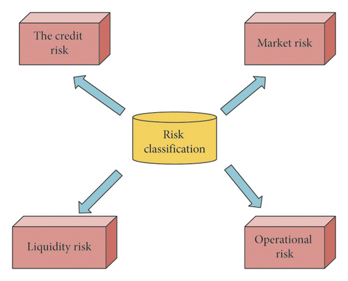
The risks faced by the financial industry are diverse [14]. Figure 1 shows some of the common risks encountered in the financial sector.

Details are in the caption following the image — Open in figure viewer PowerPoint

In the financial sector, usually, ML techniques are introduced to predict the risks. The ML techniques optimize model performance through training set and training model and then analyze and process other data [15]. In the initial ML-based model development stage, the research focuses on the execution ability of the system and adjusts the machine parameters to adapt to different data conditions. After continuous development, machines simulate human learning principles and study different ML strategies and methods by integrating the knowledge of many different subjects. Through the integration of different learning methods, the concept of integrated learning is formed and combined with artificial intelligence (AI), which attracts great attention in the field of prediction and classification [16]. Several classification algorithms have been utilized to optimize consumer finance and online business. The following section provides an overview of the commonly used ML algorithms to detect fraudulent credit card transactions.

2.1.1. Logistic Regression (LR)

LR is a simple algorithm in ML, and an intuitive classical algorithm as well, which is generally used in binary classification. In real life, there are many secondary classification problems: judging the authenticity of the received e-mail, judging whether the condition has deteriorated, and whether the borrower can repay [17]. For the binary classification problem, the target variable of LR is 1 or 0. In the linear regression model, the target variables are generally continuous. In the logical regression, the target value of the final expected output is discrete, that is, 0 or 1. Therefore, based on the results of LR, logical regression uses the activation function to map the continuous output between 0 and 1 and convert it into a concept, achieving the binary classification. LR can be used in many fields because of its simple form and strong interpretability [18].

2.1.2. Decision Tree (DT)

It is an inductive classification algorithm based on instance category and an important data classification method. It can help to build a decision tree model based on the relevant dataset and summarize the simple and clear classification method by the recursive classification principle from high to low. First, the attribute classification measurement is used to find the root node, use the same principle to divide the sub-dataset, and build the terminal leaf node. Each leaf node is recorded as a category. The relevant path is transmitted from the root node to the path and the leaf node according to the classification data or classification rules. The main task is to judge whether consumers will breach the contract, which is a problem of two categories. Therefore, the number of decisions based on the task of two categories is briefly introduced below. Here, the principle of the algorithm is described according to the relevant characteristics of males and females. The decision process is shown in Figure 2.

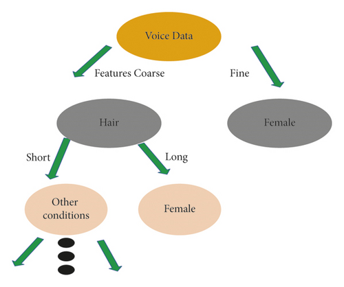
Figure 2 shows that a person’s gender is recognized by his voice and his hairstyle in the next link. The whole process is a binary tree structure. In the above DT, each nonleaf node has an attribute and the key to building DT is to select an appropriate feature attribute and classify it in different forms according to the different features. After the construction of the DT, the decision should be trimmed to improve the generalization ability of the model [19].

2.1.3. Support Vector Machine (SVM)

It is a widely used binary classification model. It is based on the theory that the linear classifier maximizes the interval of data in the feature space. It can also use the kernel function to map the input to the high-dimensional space for nonlinear classification [20]. When the information is linearly separable, dataset D is recorded as

(1)

where X_i and Y_i are category labels. The ultimate goal of SVM is to find the best line and hyperplane and minimize the classification error on the relevant datasets. In general, SVM uses the interval maximization method to obtain the best line and hyperplane. A linearly separable hyperplane can be expressed as

(2)

where ω is the weight vector and b is the offset. The boundary H₁ of the interval defined by hyperplane H₂ is computed as

(3)

(4)

The training tuples that fall on hyperplanes H₁ and H₂ are called support vectors. This is essentially a problem of solving convex quadratic optimization, and its objective function can be expressed as

(5)

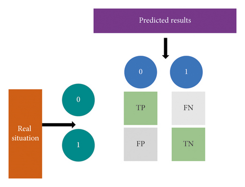
When the result of the classification algorithm is evaluated, the influence of the confusion matrix on it is significant. It is the calculation core of the classification algorithm. Its specific process is shown in Figure 3.

Figure 3 shows the four parameters of the confusion matrix. Their meanings are as follows: true positive (TP) represents the real case, and it means the group of positive elements correctly classified by the classifier. True negative (TN) represents the true negative case, which means the negative tuple is accurately divided by the classifier. False positive (FP) represents the false-positive case, and it means negative tuples that are not accurately divided into positive tuples by the classifier. Positive (P) is the number of positive tuples, and negative (N) is the number of negative tuples [20]. False negative (FN) represents a false-negative case, and it means that the positive element group is not correctly divided into negative tuples by the classifier. The evaluation index of the classification model can be deduced with the parameters. Accuracy, also known as overall recognition rate, shows whether the classification model can normally identify each dataset. Precision shows the proportion of the classification results of each category in the classification model and objectively reflects the accuracy of judging each category. The recall is also called sensitivity, and it can show the response of the classification model to each category dataset and the proportion that can be recognized by the classification model in the data. Because the relationship between precision and recall is negatively correlated, the harmonic mean value of the two is regarded as another index to reflect the overall status of the model. The value range of this index is between 0 and 1. The larger the number is, the better the overall performance is, which is expressed by the F1 score (F1). The evaluation indexes of the four classification models are expressed as

(6)

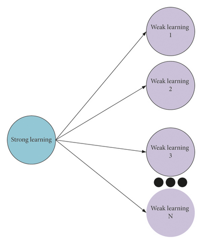
The characteristic of ensemble learning (EL) is to learn from each other [21]. The principle of the integrated algorithm is to integrate different algorithm models reasonably. Then, the comprehensive classification level of datasets in the model is improved. The methods mentioned here include bagging and boosting. The most important bagging strategy is to fuse the results of multiple base classifiers and find the final classification of the overall model by voting, which can improve the stability of classification [22]. In base classifier training, the relevant data of samples are found through the strategy of putting back sampling to form the training dataset of base classifiers. The reason for this is to reduce the correlation between base classifiers and make base classifiers have the ability to judge and think independently. The principle of EL is shown in Figure 4.

Boosting strategy theory is to continuously improve the recognition and division performance of invalid samples and realize the improvement of the comprehensive classification performance of the model. This strategy is trained in sequence in the process of training the base classifier. The last classifier classifies unreasonable samples, and the weight value of the sample data is increased in the later classifier training. In this process, the invalid division of samples by the model is continuously reduced, and the performance of the model is improved [23]. The integration methods associated with this algorithm are briefly introduced.

2.2. Classification Method Based on EL

2.2.1. Random Forest (RF)

The classification process of the RF algorithm is shown in Figure 5.

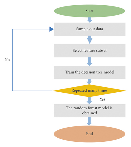
The classification results of the RF model are closely related to the performance of related DTs. If the classification performance of individual DT is good, the comprehensive classification performance is better. Moreover, the performance of RF is related to the correlation degree of two RFs in the model. The higher the correlation degree between two RFs is, the greater the possibility of errors is [24]. The correlation degree of DT is related to the number of feature m. When m is large, the correlation between them is stronger. In the RF model, the bootstrap method is used, so the data that are not taken are the out-of-bag error rate calculation samples of the RF model. The calculation process of out-of-bag error rate is divided into three steps: the first step is to calculate the samples of out-of-bag error rate and deduce the classification results of R. Then, the most relevant items in the tree voting results are used to obtain the final result of sample classification. In other words, the out-of-bag error rate refers to the ratio of the number of wrong samples to the total samples. The out-of-bag error rate is an unbiased estimation of the RF generalization error [25].

2.2.2. Gradient Boosting Decision Tree (GBDT)

With the development of digital technology, the integration of algorithms is the main process in the financial field. GBDT is one of the most commonly used integration algorithms. The implementation of the algorithm includes eXtreme Gradient Boosting (XGBoost) and LightGBM because the data processed are very complex. XGBoost is developed by Friedman and used for classification and regression. The principle of GBDT is to let all learners in gradient boosting (GB) regress the decision tree based on the classification and regression tree (CART). During the iteration of the model, sub-models are added, and it is necessary to ensure that the sample loss function decreases continuously during the iteration. GBDT can select many loss functions and consider the weight of the regression tree when solving classification problems, which makes the training effect better and the generalization ability better. Because there is a little dependency between the learners in the ladder lifting DT algorithm, it cannot be processed in parallel and the data features, but the algorithm still has some room for improvement. Therefore, the limit gradient lifting algorithm is improved on the GBDT. After the tree models are integrated, the limit gradient lifting algorithm obtains a classifier with strong performance, so that the algorithm has a stronger prediction effect and better classification accuracy. The limit gradient lifting algorithm runs multithreading through the computer central processing unit (CPU) so that GBDT can be implemented efficiently. Compared with GBDT, the gradient limit lifting algorithm uses the first derivative information and Taylor’s second-order expansion to deal with the loss function, which greatly improves the accuracy and efficiency of the model. When XGBoost processes large and complex data, it faces many difficulties and challenges, such as complex calculation and long-time consumption, which restrict the performance of the algorithm [26].

The gradient lifting DT algorithm and the limit gradient lifting algorithm are time-consuming and difficult to analyze the characteristics of complex data. In this case, LightGBM is introduced. It is the fusion of gradient single-sided sampling algorithm and feature binding algorithm. These two algorithms solve two important problems: the number of data and the number of data features.

The gradient single-sided sampling algorithm considers that the sample points with a large gradient can provide more information gain, so the gradient single-sided sampling algorithm will save the data with a large gradient and sample the sample points with a small gradient according to a certain proportion. It reduces the time complexity by reducing the number of samples, and the feature binding algorithm reduces the complexity by reducing the number of features. Usually, the data used will not be 0 at the same time; that is, they are mutually exclusive. Feature bundling algorithm is to reduce the number of mutually exclusive features by bundling mutually exclusive features. The LightGBM can identify mutually exclusive features and bundle them into a single feature so that the complexity is lowered.

2.3. Construction of Financial Risk Prediction Algorithm

LightGBM is built based on DT and histogram algorithms, which make it easier to segment data. Compared with the previous DT model, the direction of LightGBM is vertical; that is, LightGBM generates DT leaves, and other DT models generate tree levels, so the running speed of LightGBM can be better and less. Its main feature is to make the attribute discrete as floating-point continuous variables, and k discrete data are constructed into a histogram. The specific width of the histogram is k, and the number of discrete values gathered in each histogram is obtained. In the subsequent classification process, the optimal segmentation point can be obtained according to the width of the histogram. The idea of the histogram is to convert floating-point data into binary data. The detailed operation is to determine the number of barrels covered in each feature, divide equally, and then update the data of each barrel. The principle of LightGBM is shown in Figure 6. Compared with other DT algorithms, LightGBM runs faster and has little memory, and its accuracy is not affected by other factors, so speed and accuracy can be merged at the same time [27].

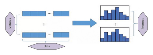
In the process of building the ML model, the dataset needs to be divided into training sets and test sets [28]. The training set is used to train the model, and the test set is used to evaluate the performance of the model. The training set is trained by the 5-fold cross-validation method, which randomly divides the data into 5 parts to ensure that the proportion of data samples does not change [29]. Four parts are randomly selected as the training set of the model, and the fifth part is used as the test set. The process is repeated until data become the test set of the model. After five cycles, the average prediction results of the five training models are calculated, and the final prediction results of the model are obtained. The feature sampling rate of LightGBM is set to 0.375, and the learning rate is set to 0.02.

2.4. Dataset Preparation

The data in this study are obtained from Alibaba Cloud Tianchi big dataset, and they are the loan records in relevant lending platforms. There are about 800000 samples in the dataset. The dataset contains 47 customer information indexes, 46 explanatory variables, and 1 target variable. The types of explanatory variables are shown in Figure 7.

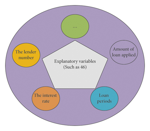
The data obtained have many problems, such as data inconsistency, data redundancy, and data imbalance. The integrity and rationality of the data have a great impact on the final performance of the model, so we need to preprocess the data [30]. The data preprocessing mainly includes several points, as shown in Figure 8.

The data preprocessing methods are described in detail as follows:

(i)
Missing Value Handling. In the process of data acquisition, human factors or computer factors may not be collected, resulting in missing values. Generally, if some data do not exist, they can be identified as missing values. When the data are missing, there are generally three methods: deleting the missing value sample data; modeling directly on data with missing values; and using statistics to fill the corresponding value. Usually, the accuracy of the model is optimized by using the missing value of fitting to make up the difference.
(ii)
Outlier Handling. In the initial dataset, there are usually a few data distributions that deviate from expectations or differ from other data distributions. These data are outliers. Outliers will lead to the increase of error variance, and the overfitting ability of the model will also be affected. Therefore, the judgment and output of outliers are important in data preprocessing. Methods such as deletion, conversion, and filling can be used. In consumer financial analysis, outliers can be regarded as risks [31].
(iii)
Data Transformation. The types of data can generally be divided into the numerical type and the nonnumerical type. Nonnumerical data can be converted into numerical types that can be processed by data coding, and then the model is constructed. In the initial data, the data to be converted include date variables, loan grade, and other variables with a certain order.

In ML, if the number of samples of different classifications of target variables in the training set is averaged, the predictability of the ML model trained with an average dataset will be better. In reality, datasets generally do not have such an ideal situation, and usually, there is a large gap in the number of samples in different categories. Unbalanced data samples have negative impacts on the model, resulting in poor classification results. In the unprocessed dataset, the number of samples without a default is positive and negative, and the distribution of samples is 4 : 1, which is unbalanced data, so it is necessary to balance the data.

In dealing with the problem of data imbalance, more resampling techniques are used to optimize the model by undersampling and oversampling. Undersampling is to reduce the number of samples of most classes to achieve the balance of samples. This method has its limitations. When the categories with a large number of samples are deleted, data information will be lost. Oversampling is to achieve sample equalization by adding a small number of samples. Generally, random oversampling and synthetic minority oversampling technology (SMOTE) is used [32]. Several samples are randomly selected according to an appropriate proportion. This method will increase the number of repeated data and lead to a small degree of data variation, and the prediction ability of the model will deteriorate. In this study, SMOTE is used to deal with data imbalance. The core steps of SMOTE are three steps. In the first step, the k-nearest neighbors are used to obtain the k-nearest neighbors of all samples in a few classes. In the second step, the few samples are specified as X, and the relevant samples that are randomly selected from the k-nearest neighbors are y. The third step is to study randomly obtained nearest neighbor y and set up a new sample according to the following equation:

(7)

where rand is a random number. After the data are balanced, the initial data volume changes from 800000 to 12823451, and the proportion of positive and negative samples after balance is 1 : 1.

2.5. Model Evaluation Indexes

After the model is constructed, different indexes need to be used to evaluate the performance of the model. The main evaluation indexes of the recognition model include prediction accuracy, precision, and recall. Their functions are as follows: prediction accuracy is an index to measure the overall performance of the algorithm, precision is an index to measure the precision rate, and recall is a metric to measure the recall rate. These indexes are computed as

(8)

(9)

(10)

Among the above three evaluation indexes, T_P is the number of positive samples when positive samples are predicted, T_n is the number of negative samples predicted as negative samples, F_P is the number of negative samples predicted as positive samples, and F_n represents the number of positive samples predicted as negative samples.

3. Results

3.1. Comparison of Indexes of Different Prediction Algorithms

The designed LightGBM prediction model is trained with the balanced dataset, and the performance is compared with the DT and RF algorithms on the test set. The comparative results are shown in Figure 9.

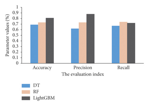
Figure 9 shows that the accuracy rate of the LightGBM prediction model is 81%, the precision is 88%, and the recall rate is 72%. Similarly, the accuracy of DT is 68%, the precision is 60%, and the recall is 67%. Likewise, the accuracy rate of RF with similar performance is 73%, the precision is 73%, and the recall rate is 74%. In general, the performance effect of the LightGBM model in loan classification is better than other traditional ML models.

3.2. Performance Comparison of Different Algorithms

The area under the curve (AUC) represents the degree or measure of separability. F1 score (F1) is an index to evaluate the accuracy of the binary classification model. The larger the AUC and F1 are, the better will be the performance of the model. The AUC and F1 values of LightGBM, DT, and RF are obtained from the test set and are shown in Figure 10.

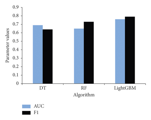
From the AUC value distribution of different algorithms, the AUC value of LightGBM L is 0.76, that of DT is 0.69, and that of RF is 0.65. From the F1 values, the F1 value of LightGBM is 0.79 as compared to the F1 value of DT and RF which are 0.63 and 0.70, respectively. The F1 value of LightGBM is closer to 1, which is the largest. This shows that the performance of LightGBM is better and LightGBM can better classify and predict whether an individual default or not.

4. Conclusion

Inspired by the market economy and the growth of the Internet loan financial industry, the service subject of consumer finance becomes gradually complex and has become a significant factor for endorsing the development of the industrial economy in the financial sector. Because economic enterprises are experiencing huge and sustained economic losses, and in view of the increasing difficulty of detecting personal default, it is of great significance to develop more effective methods for detecting personal default required by new financial enterprises. This study proposed a novel approach for predicting individual default and preventing default in consumer finance using an improved LightGBM algorithm. We conducted numerous experiments using the Alibaba Cloud Tianchi big dataset. First, several traditional ML methods were systematically introduced, their advantages and disadvantages were examined, the principle of LightGBM was described, and the key factors affecting the performance of LightGBM were discussed. Second, the prediction performance of LightGBM was optimized. The optimization greatly improved the prediction accuracy of personal default that helps to effectively analyze the complexity of consumer finance, decrease the investment risk of the financial industry, and promote the progress of the industrial economy in the field of consumer finance. Finally, the performance of the proposed method and other state-of-the-art ML algorithms were tested and compared. The experimental result shows that LightGBM performed better than other traditional ML models in loan classification. However, there are still some shortcomings such as the size of the samples being small, which may have an impact on the experimental results. In future research, we will focus on the listed limitation.

Conflicts of Interest

The authors declare that there are no conflicts of interest regarding the publication of this paper.

Acknowledgments

The study was supported by “Research on Guangxi Financial Development Promoting Economic Transformation and Upgrading Path Under New Economic Era” (Beibu Gulf University, Project no. 2016PY-SJ19) and “Research on Financial Support for the Transformation and Upgrading of Small and Medium-sized Private Enterprises in Guangxi”(Education Department of Guangxi Zhuang Autonomous Region, Project no. 2018KY0585).

Open Research

Data Availability

The data used to support the findings of this study are available from the corresponding author upon request.

References

1 Chi M. T. H, Adams J, Bogusch B. E., Kang S, Lancaster M, Levy R, Li N, Eldoon K. L. M, Stump G. S, Wylie R, Xu D, and Yaghmourian D. L, Translating the ICAP theory of cognitive engagement into practice, Cognitive Science. (2018) 42, no. 6, 1777–1832, https://doi.org/10.1111/cogs.12626, 2-s2.0-85051736513.
10.1111/cogs.12626
Web of Science® Google Scholar
2 Boutaba R, Salahuddin M. A, Limam N., Ayoubi S, Shahriar N, Solano F. E, and Caicedo O. M, A comprehensive survey on machine learning for networking: evolution, applications and research opportunities, Journal of Internet Services and Applications. (2018) 9, no. 1, 1–99.
10.1186/s13174-018-0087-2
Web of Science® Google Scholar
3 Pacheco F., Exposito E., Gineste M., Baudoin C., and Aguilar J., Towards the deployment of machine learning solutions in network traffic classification: a systematic survey, IEEE Communications Surveys & Tutorials. (2019) 21, no. 2, 1988–2014, https://doi.org/10.1109/comst.2018.2883147, 2-s2.0-85057431136.
10.1109/COMST.2018.2883147
Web of Science® Google Scholar
4 Massaro A., Maritati V., and Galiano A., Data Mining model performance of sales predictive algorithms based on RapidMiner workflows, International Journal of Computer Science and Information Technology. (2018) 10, no. 3, 39–56, https://doi.org/10.5121/ijcsit.2018.10303.
10.5121/ijcsit.2018.10303
Google Scholar
5 Rafiei M. H. and Adeli H., A new neural dynamic classification algorithm, IEEE Transactions on Neural Networks and Learning Systems. (2017) 28, no. 12, 3074–3083, https://doi.org/10.1109/tnnls.2017.2682102, 2-s2.0-85021652833.
10.1109/TNNLS.2017.2682102
PubMed Web of Science® Google Scholar
6 Wan X., Jin Z., Wu H., Liu J., Zhu B., and Xie H., Heartbeat classification algorithm based on one-dimensional convolution neural network, Journal of Mechanics in Medicine and Biology. (2020) 20, no. 07, 2050046, https://doi.org/10.1142/s0219519420500463.
10.1142/S0219519420500463
Web of Science® Google Scholar
7 Leo M., Sharma S., and Maddulety K., Machine learning in banking risk management: a literature review, Risks. (2019) 7, no. 1, https://doi.org/10.3390/risks7010029, 2-s2.0-85064808150.
10.3390/risks7010029
Web of Science® Google Scholar
8 Jaroszewski A. C., Morris R. R., and Nock M. K., Randomized controlled trial of an online machine learning-driven risk assessment and intervention platform for increasing the use of crisis services, Journal of Consulting and Clinical Psychology. (2019) 87, no. 4, 370–379, https://doi.org/10.1037/ccp0000389, 2-s2.0-85063303480.
10.1037/ccp0000389
PubMed Web of Science® Google Scholar
9 Carcillo F., Dal Pozzolo A., Le Borgne Y.-A., Caelen O., Mazzer Y., and Bontempi G., SCARFF: a scalable framework for streaming credit card fraud detection with spark, Information Fusion. May 2018, 41, 182–194, https://doi.org/10.1016/j.inffus.2017.09.005, 2-s2.0-85029580394.
10.1016/j.inffus.2017.09.005
Web of Science® Google Scholar
10 Yuan S., Wu X., Li J., and Lu A., Spectrum-based deep neural networks for fraud detection, Proceedings of the ACM on Conference on Information and Knowledge Management, November 2017, Singapore.
Google Scholar
11 Dhankhad S., Mohammed E., and Far B., Supervised machine learning algorithms for credit card fraudulent transaction detection: a comparative study, Proceedings of the. IEEE Int. Conf. Inf. Reuse Integr. (I), July 2018, Salt Lake City, UT, USA, 122–125, https://doi.org/10.1109/IRI.2018.00025, 2-s2.0-85052334316.
10.1109/IRI.2018.00025
Google Scholar
12 Dal Pozzolo A., Boracchi G., Caelen O., Alippi C., and Bontempi G., Credit card fraud detection and concept-drift adaptation with delayed supervised information, Proceedings of the Int. Joint Conf. Neural Netw. (IJCNN), July 2015, Killarney, Ireland, 1–8, https://doi.org/10.1109/IJCNN.2015.7280527, 2-s2.0-84951012186.
10.1109/IJCNN.2015.7280527
Google Scholar
13 Taha A. A. and Malebary S. J., An intelligent approach to credit card fraud detection using an optimized light gradient boosting machine, IEEE Access. (2020) 8, 25579–25587, https://doi.org/10.1109/access.2020.2971354.
10.1109/ACCESS.2020.2971354
Web of Science® Google Scholar
14 de Sá A. G. C., Pereira A. C., and Pappa G. L., A customized classification algorithm for credit card fraud detection, Engineering Applications of Artificial Intelligence. (2018) 72, 21–29, https://doi.org/10.1016/j.engappai.2018.03.011, 2-s2.0-85044505936.
10.1016/j.engappai.2018.03.011
Web of Science® Google Scholar
15 Keck T., FastBDT: a speed-optimized multivariate classification algorithm for the Belle II experiment, Computing and Software for Big Science. (2017) 1, no. 1, https://doi.org/10.1007/s41781-017-0002-8.
10.1007/s41781-017-0002-8
Google Scholar
16 Burton J. W., Stein M. K., and Jensen T. B., A systematic review of algorithm aversion in augmented decision making, Journal of Behavioral Decision Making. (2020) 33, no. 2, 220–239, https://doi.org/10.1002/bdm.2155.
10.1002/bdm.2155
Web of Science® Google Scholar
17 Zhang H., Khurshid A., Xinyu W., and BĂLTĂŢEANU A. M, Corporate financial risk assessment and role of Big data; New perspective using fuzzy analytic hierarchy process, Journal for Economic Forecasting. (2021) 2, 181–199.
Google Scholar
18 Blazquez D. and Domenech J., Big data sources and methods for social and economic analyses, Technological Forecasting and Social Change. (2018) 130, 99–113, https://doi.org/10.1016/j.techfore.2017.07.027, 2-s2.0-85028816304.
10.1016/j.techfore.2017.07.027
Web of Science® Google Scholar
19 Saggi M. K. and Jain S., A survey towards an integration of big data analytics to big insights for value-creation, Information Processing & Management. (2018) 54, no. 5, 758–790, https://doi.org/10.1016/j.ipm.2018.01.010, 2-s2.0-85041554154.
10.1016/j.ipm.2018.01.010
Web of Science® Google Scholar
20 Oussous A., Benjelloun F. Z., Ait Lahcen A., and Belfkih S., Big data technologies: a survey, Journal of King Saud University-Computer and Information Sciences. (2018) 30, no. 4, 431–448, https://doi.org/10.1016/j.jksuci.2017.06.001, 2-s2.0-85020839077.
10.1016/j.jksuci.2017.06.001
Web of Science® Google Scholar
21 Abdel-Basset M., Mohamed M., and Chang V., NMCDA: a framework for evaluating cloud computing services, Future Generation Computer Systems. (2018) 86, 12–29, https://doi.org/10.1016/j.future.2018.03.014, 2-s2.0-85043606484.
10.1016/j.future.2018.03.014
Web of Science® Google Scholar
22 Varghese B. and Buyya R., Next-generation cloud computing: new trends and research directions, Future Generation Computer Systems. (2018) 79, 849–861, https://doi.org/10.1016/j.future.2017.09.020, 2-s2.0-85030685680.
10.1016/j.future.2017.09.020
Web of Science® Google Scholar
23 Benitez J., Ray G., and Henseler J., Impact of information technology infrastructure flexibility on mergers and acquisitions, MIS Quarterly. (2018) 42, no. 1, 25–43, https://doi.org/10.25300/misq/2018/13245, 2-s2.0-85041231903.
10.25300/MISQ/2018/13245
Web of Science® Google Scholar
24 Korol I. and Poltorak A., Financial risk management as a strategic direction for improving the level of economic security of the state, Baltic Journal of Economic Studies. (2018) 4, no. 1, 235–241, https://doi.org/10.30525/2256-0742/2018-4-1-235-241.
10.30525/2256-0742/2018-4-1-235-241
Google Scholar
25 Valaskova K., Kliestik T., Svabova L., and Adamko P, Financial risk measurement and prediction modelling for sustainable development of business entities using regression analysis, Sustainability. (2018) 10, no. 7, https://doi.org/10.3390/su10072144, 2-s2.0-85048952033.
10.3390/su10072144
Web of Science® Google Scholar
26 Kim A., Yang Y., Lessmann S., Ma T., Sung M. C., and Johnson J., Can deep learning predict risky retail investors? A case study in financial risk behavior forecasting, European Journal of Operational Research. (2020) 283, no. 1, 217–234, https://doi.org/10.1016/j.ejor.2019.11.007.
10.1016/j.ejor.2019.11.007
Web of Science® Google Scholar
27 Yang Q., Wang Y., and Ren Y., Research on financial risk management model of internet supply chain based on data science, Cognitive Systems Research. (2019) 56, 50–55, https://doi.org/10.1016/j.cogsys.2019.02.001, 2-s2.0-85063398345.
10.1016/j.cogsys.2019.02.001
Web of Science® Google Scholar
28 Brooks C., Sangiorgi I., Hillenbrand C., and Money K., Experience wears the trousers: exploring gender and attitude to financial risk, Journal of Economic Behavior & Organization. (2019) 163, 483–515, https://doi.org/10.1016/j.jebo.2019.04.026, 2-s2.0-85066271368.
10.1016/j.jebo.2019.04.026
Web of Science® Google Scholar
29 Nguyen L., Gallery G., and Newton C., The joint influence of financial risk perception and risk tolerance on individual investment decision-making, Accounting and Finance. (2019) 59, no. S1, 747–771, https://doi.org/10.1111/acfi.12295, 2-s2.0-85028755568.
10.1111/acfi.12295
Web of Science® Google Scholar
30 Sathyamoorthi C., Mapharing M., Mphoeng M., and Dzimiri M., Impact of financial risk management practices on financial performance: evidence from commercial banks in Botswana, Applied Finance and Accounting. (2019) 6, no. 1, https://doi.org/10.11114/afa.v6i1.4650.
10.11114/afa.v6i1.4650
Google Scholar
31 Myšková R. and Hájek P., Mining risk-related sentiment in corporate annual reports and its effect on financial performance, Technological and Economic Development of Economy. (2020) 26, no. 6, 1422–1443, https://doi.org/10.3846/tede.2020.13758.
10.3846/tede.2020.13758
Web of Science® Google Scholar
32 Alshehhi A., Nobanee H., and Khare N., The impact of sustainability practices on corporate financial performance: literature trends and future research potential, Sustainability. (2018) 10, no. 2, https://doi.org/10.3390/su10020494, 2-s2.0-85041928796.
10.3390/su10020494
Web of Science® Google Scholar

Citing Literature

All articles

[Retracted] Complexity Analysis of Consumer Finance following Computer LightGBM Algorithm under Industrial Economy

Retraction(s) for this article

Retracted: Complexity Analysis of Consumer Finance following Computer LightGBM Algorithm under Industrial Economy

Abstract

1. Introduction