For the purpose of simultaneously estimating and locating the linear frequency modulation (LFM) emitter with unknown parameters, an innovative approach, i.e., Fast Direct Position Determination (FDPD), is introduced. The proposed algorithm is based on maximum likelihood estimation (MLE) and spectrum detection. To improve the accuracy and overcome the dramatic complexity of plain maximum likelihood formulation, we further derive the objective function equation of Direct Position Determination (DPD) algorithm and present an enhanced strategy to solve the highly nonlinear optimization problem. By combining the two-step localization method, one-step localization method, and short-time Fourier transform (STFT), our approach realizes jointly estimation of the transmitted signal parameters and emitter localization. Simulation results show that the proposed method is superior compared to the existing DPD, and two-step localization algorithms in terms of localization error and computational complexity, especially for low signal-to-noise ratio (SNR).

1. Introduction

Localization of emitters is a fundamental demand in many application fields, such as radar [1, 2], sonar [3, 4], global navigation satellite systems (GNSS) [5, 6], wireless sensor network [7, 8], and seismic exploration [9, 10]. Linear frequency modulation (LFM) signals, known as large time-bandwidth product and high resolution signals, are frequently used in localization systems and have attracted increasing attention of many scholars. As stealth technology and low intercept technology get prosperous and mature, passive emitter localization technology has gradually developed from the traditional single station to using several widely distributed receiver stations. This paper considers a passive localization problem for an emitter by multiple diffusely separated receiver stations.

In general, the localization methods contain two main categories of two-step localization method and one-step localization method. Algorithms of two-step localization method [11–20] are commonly composed of two steps: first, each receiver station measures and computes the parameters related to the position of the target. The parameters involved in position include time difference of arrival (TDOA) [11–13], angle of arrival (AOA) [14–17], frequency difference of arrival (FDOA) [18–20], etc. The second step is to construct equations using the parameters to estimate the position of the target. Both steps of two-step method might be optimal; given their input, two-step method is still suboptimal. Since the correlation between different receiver stations is ignored, the precision of the parameter measurement in the first step is limited. Moreover, the parameters may be virtually absent in some of the receiver stations due to the signal strength fluctuation and different path attenuation, leading to data association and performance deterioration issues, especially in low signal-to-noise ratio (SNR) scenarios.

One-step localization method [21–35] processes the observed signals in the central processor without parameter extraction and then constructs the cost function only related to the position of the emitter. This kind of localization algorithms finally obtain the position of the emitter through the maximum likelihood estimation (MLE), the least squares, the grid search, gradient-based methods, etc. Therefore, it is also referred to direct position determination (DPD) [21–24]. In 2004, Weiss first proposed direct position determination technology [21], analyzed, and compared the DPD performance with AOA for signals with known (DPD-known) and unknown waveforms (DPD-unknown) [22, 23]. Over the past dozen years, multiple DPD algorithms have been presented to enhance performance of passive localization system based on different approaches including the maximum likelihood (ML) [25, 26], the time frequency analysis (DPD-STFT-w) [27], the multiple signal classification (MUSIC) [28, 29], the expectation maximization (EM-DPD) [30, 31], the minimum variance distortionless response (MVDR) [32–34], and the time-varying delay [35]. Compared with the one-step approaches, the DPD algorithms directly estimate the initial position of the target according to the received signals in the central station, avoiding the process of correlation of parameters of different receivers. Moreover, DPD can locate the signals (simultaneous signals with same frequency, etc.) which are difficult to be processed by traditional methods. At the same time, because the cost function of DPD is only related to the position of the emitter, it has higher localization accuracy and better robustness at lower SNR on account of making full use of the prior information of the signals which are coming from the same emitter [23]. However, since the DPD algorithms deal with the original sampled signals rather than the analytic solutions of the emitter, the computational complexity increases rapidly and the estimation performance of waveform parameters deteriorates drastically when the SNR is lower than a threshold point, i.e., the “threshold effect.”

This paper addresses passive localization of an LFM emitter with unknown signal parameters. Aiming at the problem of “threshold effect” and high computational complexity of DPD algorithms at low SNR, we proposed a Fast Direct Position Determination (FDPD) algorithm. The proposed algorithm can realize the combination of emitter localization and parameter estimation of the LFM signal. The main procedures of this approach include the following:

(i)
Firstly, the signal spectrum is obtained through short-time Fourier transform (STFT) and other operations (linear fitting, the least square method, etc.); then, the SNR is calculated
(ii)
Compared the SNR with the threshold point, the cooperative localization of two-step method and one-step method is combined to finally achieve the optimal localization. The performance of the two-step method and one-step method is similar at high SNR, we choose the two-step method owing to its less computational complexity. Chan algorithm [36] and Taylor algorithm [37], which are two representative algorithms of two-step localization method, are selected to complete collaborative localization: Chan algorithm is used to estimate the initial position coordinates, regarding it as the initial value, and Taylor series expansion algorithm is used to obtain the further position coordinates
(iii)
At low SNR, the initial frequency, chirp rate, and other signal parameters are estimated by time frequency analysis, thus we can capture the entire parameter set of the LFM profile of the signal and obtain an objective function. Then, a four dimensional search (4D) is carried out at the position coordinates obtained by Chan and Taylor algorithms. To solve the highly nonlinear optimization problem (four-dimensional search), we turn the four-dimensional search into a two-dimensional parameter estimation combined with grid search. The search range is determined by the error analysis of Chan and Taylor algorithms. Simulation results show that the proposed algorithm reduces the computational complexity, and the positioning accuracy is better than Chan, Taylor, DPD, and other traditional algorithms

The rest of this paper is organized as follows. Section 2 introduces the model of the LFM signal for widely separated receiver stations. In Section 3, the localization problem formulated in an ML estimation paradigm is clarified. Section 4 presents the proposed FDPD algorithm in detail. Section 5 provides the numerical simulations. The conclusions are drawn in Section 6.

2. Signal Model

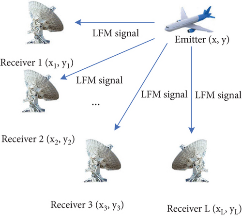
Consider a 2D Cartesian coordinate system where a noncooperative stationary emitter transmitting signals. We let the vectors p_l(x_l, y_l), (l = 1, 2, ⋯, L) represent the positions of L widely separated receiver stations. The transmitter position is denoted by the vector of coordinates p(x, y). As shown in Figure 1, the emitter transmitted an LFM signal s(t). Then, the signal is intercepted by the receiver stations and transmitted to the center processor.

Details are in the caption following the image — **Figure 1**
Open in figure viewer PowerPoint

Sketch map of an emitter and L widely distributed receiver stations.

The LFM signal is modeled as

(1)

where f₀ denotes the initial frequency of the LFM signal, k is the chirp rate, and T_p is the time duration. The signal observed by the lth receiver station is given by

(2)

r_l(t) is a time-dependent vector, b_l is an unknown complex scalar representing the attenuation coefficient related with regard to the path from the emitter to the receiver stations, and α_l(p) is the lth array response to signal transmitted from position p. s(t − τ_l(p) − t₀; f₀, k, T_p) is the signal waveform, transmitted at time t₀ and delayed by τ_l(p). The vector n_l(t) represents the independent and identically distributed zero-mean complex Gaussian white noise with corvariance matrix

, and each receiving channel is independent of each other. τ_l(p) can be calculated by [35]

(3)

with c denoting the speed of light.

After sampling, the continuous signal of Equation (2) can be expressed in a vector form

(4)

where

(5)

with N_s denotes the number of the samples, f_s denotes the sampling frequency, B is the signal bandwidth, and T is the time duration of the received signal, thus N_s = T∗f_s (f_s ≥ 2B).

3. Problem Formulation about Direct Position Determination

Derived from [38], the MLE of the unknown parameter vector can be estimated by examining the likelihood ratio, with H₁ corresponding to the target-present hypothesis. When the distribution characteristics of noise

are known, MLE can be used [21, 39]. Here, we assume that

is the identically distributed zero-mean complex Gaussian white noise, with correlation matrix

. In addition, the receiver stations are distributed widely enough to warrant mutual independence of noise vectors,

(6)

According to Equation (4), we can construct the probability density function (PDF) as

(7)

where C₁ is a constant, and [.]^H represents the operation of conjugation transpose. Thus, the likelihood ratio function can be obtained as

(8)

Let ∂L(r_l)/∂b_l = 0,

, and

. Finally, we can get the maximum likelihood function as follows:

(9)

Remarkably, we observe from Equation (9) that the parameters to be estimated in the objective function include the transmitter position, the signal parameters, and the time t₀. It is a highly nonlinear optimization problem whose closed-form description of the analytic optimum solution is difficult to obtain. The numerical solution based on grid search for the region of interest is an alterative. However, the high-dimensional grid search will become computationally prohibitive when the needed localization accuracy increases. If the SNR is lower than a threshold point, the estimation errors rise quickly, i.e., the “threshold effect.” Based on the above arguments, a novel algorithm is investigated in the subsequent sections to trade off algorithm performance for implementation complexity.

4. Algorithm Description

In this section, we present a computationally efficient approach to solve a highly nonlinear optimization problem in passive localization. First, we employ STFT technique to extract the valid spectrum fragment of the transmitting signals and then further estimate the instantaneous frequency, spatial power, and other signal parameters. After extracting peak points of the power spectrum, aiming at the disadvantages of low precision of two-step method and high complexity of DPD algorithm at low SNR, we adopt corresponding objective functions to extract the emitter positions. The algorithm is described in detail below.

4.1. Estimation of Signal Parameters and Spectrum Detection

Under the circumstance of low SNR, the localization performance of DPD algorithm will deteriorate significantly. In order to improve the localization performance, in this subsection, we adopt the time-frequency analysis method to estimate the relevant parameters and detect the spectrum.

4.1.1. Parameter Estimation Based on Time Frequency Analysis

To estimate the LFM signal parameters, the most important step is to estimate instantaneous frequency (IF) from the received signal. The IF expression of the LFM signal is as follows:

(10)

After sampling,

can be written in a vector form as

(11)

where 0 ≤ α ≤ N_p − 1, and N_p is the number of samples of the LFM signal with N_p = T_p∗f_s.

As can be seen from the above equations, IF is formed by linear combination of initial frequency f₀ and chirp rate k. A large number of IF samples can be obtained through estimation, and the corresponding f₀ and k can be estimated from the IF samples by means of parameter fitting.

For the LFM signal, short-time Fourier transform (STFT) performs analysis on the signal in the time window and can intuitively reflect the trend of the frequency and the change of spectrum along with time, thus the initial frequency and chirp rate of the signal can be estimated efficiently, which has a good effect on the estimation accuracy, especially at low SNR [40–45]. The common STFT is defined as

(12)

where h(τ) is the time window function, which is called analysis window as well.

Substituting Equation (12) into the expression of the LFM signal [42], then the STFT for the LFM signal s(t) is defined as

(13)

where

(14)

By taking the square of the module of h(f), the spectrum (SP) of the LFM signal can be written in the following form:

(15)

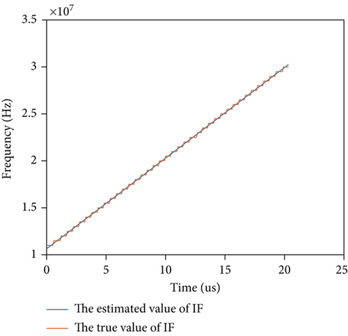
The Gaussian window is chosen as the analysis window so that |h(f)|² is a Gaussian function in essence. |h(f)|² is symmetry about the line f = 0 and achieves the maximum value at f = 0. The above formula shows that the LFM signal’s spectrum STFT_s(t, f) obtains the maximum value at frequency point f₀ + kτ at each discrete time τ. Therefore, the IF of the LFM signal can be acquired by finding the max point at each discrete time τ.

Hence, we can get the IF estimation as the following expression:

(16)

Figure 2 shows the real value and estimated value of the instantaneous frequency after linearly fitting by the least square method when SNR = −5dB. Thus, the estimated values of chirp rate and initial frequency can be calculated from the fitted straight line.

4.1.2. Extraction of the SP of the LFM Signal

The SP of the observed signal of the lth receiver station can be expressed as [38]

(17)

where n(t, f) represents the SP of noise.

After adding the moving window function h(τ), the extracted LFM signal can be written as

(18)

The SP of the LFM signal observed and extracted by the lth receiver station in Equation (17) is shown in Figure 3.

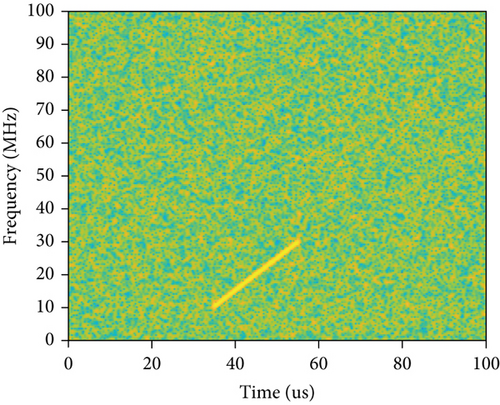
On the basis of the above process, the 2D distribution of the chirp signal’s STFT is converted into 1D relationship between frequency and time, which displays a coarse line in the time-frequency plane. It can be seen from Figure 3 that when SNR is at -5 dB, the spectral intensity of the LFM signal is much greater than that of the noise. It can be clearly seen from the figure that the time-frequency characteristics of the LFM signal reflect the sum of power spectral in each window. Summing the maximum value of spectrum of each window helps to estimate the parameters of the LFM signal and realize the spectrum detection. The localization algorithms after spectrum detection will be introduced in the subsequent sections.

4.2. The Localization Algorithm Based on Spectrum Detection

According to the “threshold effect” of DPD algorithm, the localization accuracy will deteriorate sharply when the SNR is lower than -5 dB [21]. The mean (or root mean square) of miss distance will also increase rapidly. At high SNR, DPD, Chan, Taylor algorithms have similar performance in localization, but when the SNR is lower than the threshold point, DPD methods have been demonstrated to outperform two-step methods. For most of the DPD algorithms require grid search in the final, which increases computation complexity and transmission demand in the case of lacking prior information. Therefore, Chan and Taylor algorithms are first used for coarse location. Then, grid search is carried out on the basis of the results of the coarse location, which can greatly reduce the workload. The complexity analysis will be detailed in the next subsection. The whole FDPD algorithm process is as follows.

4.2.1. Localization at High SNR

According to [46], in passive multistation localization, after obtaining TDOA measurements by Chan algorithm [13, 36], the distance differences between the emitter and the base stations are obtained, thus multiple TDOA measurements form a set of estimated equations about the emitter. We assume

is the estimated position of the emitter and (x_l, y_l), (l = 1, 2, ⋯, L) is the known position of the lth receiver station, then the emitter position can be calculated by the following formula:

(19)

where

(20)

It has been shown that the iterative algorithms (Standard least squares, hyperbolic least squares, etc.) require a definition of the initial parameters, which can significantly affect solution accuracy and computational time [47]. Therefore, to ensure the solution accuracy, the position calculated by Chan algorithm is selected for initial position (x₀, y₀) of MS for Taylor expansion of the Taylor algorithm [37]. Then, the weighted least square (WLS) method [48, 49] is used to obtain the least squares estimation of Z as follows:

(21)

where [.]^T represents the transpose operator, and φ is the covariance matrix of the measurement value of TDOA. The value of the TDOA measurements covariance matrix is estimated under the assumption that there are large numbers of samples, or equivalently, long observation time. Therefore, the Cramer-Rao matrix bound (CRMB) of the estimated TDOA vector is used to represent the value of the matrix [50].

(22)

where B is the bandwidth of the signal and tr( ^∗) is the trace of matrix ∗. S(ω) is the signal power spectrum, N(ω) = diag{N₁(ω), N₂(ω), ⋯, N_M(ω)} is the noise power spectral matrix, N_p(ω) is the lower right M − 1 by M − 1 partition of the matrix N(ω), and 1 is a vector of unity which has the same size as N_p(ω).

The selection of the initial value of iterative Taylor-series expansion method has a great influence on the location result. If the initial value is not appropriate, the Taylor algorithm will not converge. On the other hand, Chan algorithm has fast operation speed and low computation complexity. Although the Chan algorithm reduces the localization accuracy in poor channel environment, the localization results can still reflect the general characteristics between the position of the radiation source and the measured value, which is conducive to the convergence of Taylor algorithm. Therefore, we choose Chan algorithm to calculate the TDOA measured values, and the localization results of Chan algorithm are taken as the initial value of Taylor series expansion algorithm, then several iterations are carried out.

Hence, this paper adopts the collaborative localization of Chan and Taylor algorithms using Equations (19)-(22) at high SNR, which can not only ensure the small error of the initial value of the Taylor expansion, so as to ensure the localization accuracy, but also greatly reduce the amount of calculation.

4.2.2. Localization at Low SNR

When the SNR is low, the DPD algorithm is used on the basis of the location results of Chan and Taylor algorithms. To get more accurate waveform parameters, STFT is used to assist signal parameter estimation. DPD algorithm can obtain better localization accuracy on the basis of more accurate signal parameters estimation. In order to obtain more accurate positions, here, an objective function is constructed for grid search.

The IF of the LFM signal is estimated from Equation (16), so as to estimate the initial frequency and chirp rate, and then substituted into the following function, which describes the fitting error per unit time at different positions, window width, and starting time, the function is given by

(23)

where 0 ≤ α ≤ N_s − 1, N_s is the number of samples.

is referred to the minimum cost function, thus F(r, p, t₀, T_p) denotes the mean minimum cost function, i.e., the fitting error per unit time at different positions. From Equation (15),

represents the total likelihood ratio function of the signal, which reflects the sum of spectral power in all windows.

reflects the summation of the maximum SP within the sliding window. To obtain higher parameter estimation accuracy, the following objective function is defined:

(24)

Compared with the function in Equation (9), the objective function includes more factors of indicating the parameter estimation by means of STFT, which is maximized by F(r, p, t₀, T_p). Then through grid search, we can estimate the emitter position p, initial time t₀, and signal pulse width T_p more accurately. In most instances, four-dimensional search cannot be considered as a viable solution to solve a highly nonlinear optimization problem. Therefore, we used an efficient decoupled strategy to solve the problem. The basic idea of the strategy is to turn the four-dimensional search into a two-dimensional parameter estimation combined with grid search. Specifically, based on STFT, a two-dimensional estimator is firstly designed to extract the initial frequency f₀ and chirp rate k of the LFM signal in the time-frequency domain. Then, a four-dimensional search, including the previously estimated waveform parameters, is carried out, and the position of the emitter, the corresponding transmitted time, time duration, and initial frequency can be obtained by the search.

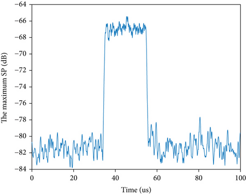
For determining when and which method should be used, that is, to decide whether the emitter signal is in high or low SNR environment, Equation (15) in 4.1.1 can be utilized. By means of maximizing the spectrum at each window, it can be seen that the maximum spectrum of the LFM signal is obviously different from the maximum spectrum of the noise. The spectrum difference between the LFM signal and the noise can be calculated and then compared with the threshold point to determine whether the emitter signal is at high or low SNR. The simulation diagram of the maximum spectrum value changing over time is shown in Figure 4.

The general pseudocodes of the proposed FDPD algorithm are shown in Algorithm 1.

Algorithm 1: Summary of the FDPD Algorithm.

Input: The observed signal r, the base station coordinates, space of grid search (N_x × N_y) for p;
Output: Estimated parameters and the position of the radiation source;
1: For l =1 ··· L do
2: Compute the SP for lth observed signal.
3: Compute the maximum SP of the lth observed signal
4: Compare the maximum SP difference between the LFM
5: Signals and noise signal with the threshold value.
6: End for
7: If the maximum SP difference > threshold then
8: Compute the emitter position p using Equation (19)–(22).
9: End if
10: If the maximum SP difference < threshold then
11: For l =1 ··· L do
12: Compute the emitter position initial ^p₁ using
13: Equation (19) - (22).
14: Determine the search range (N_x × N_y) by the
15: Error analysis of Chan and Taylor algorithm.
16: For i = 1 ⋯ (N_x × N_y) do
17: Estimate the IF of the lth observed signal using Equation (16).
18: Estimate the initial frequency and chirp rate.
19: Extract the IF and compute the fitting error every time
20: Window per unit time at different position.
21: Compute the objective function value using Equation (24).
22: Find the maximum of the objective function and compute the
23: Emitter position p.
24: End for
25: End for
26: End if

5. Simulation Results

In this section, simulations are brought forward to verify the performance of the proposed algorithm. Four receiver stations used in the simulation are located at (0,0)m (m denotes meter), (6000,0)m, (6000,6000)m, and (2400,6000)m, respectively. The approximate coordinates of the radiation source are (6000,4500)m. We perform extensive Monte Carlo simulations. In the following analysis, the results are collected and processed by averaging M Monte Carlo experiments. Simulation parameters are shown in Table 1, where M is the number of Monte Carlo experiments.

Table 1. Simulation signal parameters.

LFM signal parameter	Parameter values
Pulse width	20 μs
Band width	20 MHz
Sampling frequency	100 MHz
Initial frequency	10 MHz
Chirp rate	1 MHz/μs

For each Monte Carlo experiment, we assume that the error between the estimated position

of the emitter and the actual position (x, y) is calculated as follows:

(25)

where p_i is the estimation of p of the ith Monte Carlo trial.

The mean error (ME) of the estimated position is obtained by the statistics of M Monte Carlo experiments. ME is defined as

(26)

The root mean square error (RMSE) of the estimated parameters is defined as

(27)

where θ denotes the parameter to be estimated, such as chirp rate and initial frequency.

5.1. Analysis of Simulation Results

In Figure 3, we extract the 1D frequency-time curve of the LFM signal based on STFT and perform STFT on the transmitted signalr_l(t), the spectrum of which is symmetry aboutf = 0. In order to get the SNR for spectrum detection, according to in Equation (18), the amount of maximum SP within the sliding window can be viewed as a factor of SP. The simulation of the variation of the maximum SP in each STFT window with time is shown in the following figure.

It can be seen from Figure 4 that when the SNR is -15 dB, the maximum SP value of the LFM signal is obviously different from the maximum SP value of the noise signal. Then, the SP differential is calculated and compared with the threshold point to determine the signal environment.

Figures 5 and 6 are simulation comparison diagrams of FDPD and common direct localization algorithms.

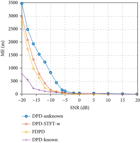
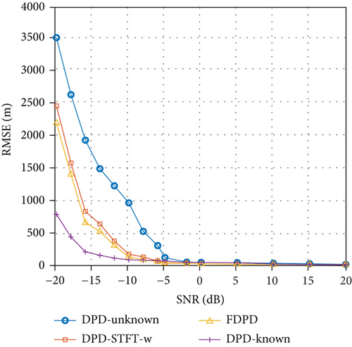
As can be seen from Figures 5 and 6, the DPD-known algorithm can acquire the optimal localization performance for the case that the transmitted signal is completely known to the receivers. Therefore, the performance of DPD-known can be viewed as an upper bound for other algorithms. Moreover, in high SNR environment, namely, higher than 0 dB, all the four algorithms achieve superior localization accuracy and perform nearly equally. When the SNR is below the threshold point, the ME and RMSE of these algorithms rise quickly as SNR decreases. As SNR decreases, the accuracy of the DPD-unknown deteriorates rapidly. When the emitter signal is unknown, FDPD and DPD-STFT-w algorithm has better localization accuracy compared with DPD-unknown algorithm, which can ensure the accuracy that the RMSE is less than 100 m when the SNR is above -5 dB. However, considering the extremely high computational complexity of DPD algorithms (DPD-STFT, EM-DPD, etc.), Chan and Taylor algorithms are used for coarse localization, and parameters are estimated on the basis of them, then the objective function is maximized by using the estimated parameters which are more accurate. This will greatly reduce the amount of calculation, so it is called fast DPD (FDPD) algorithm. The complexity analysis of FDPD algorithm and DPD, DPD-known and DPD-STFT-w algorithms will be described in detail in the next section.

5.2. Analysis of Complexity

The complexity of Chan and Taylor algorithms is O(n²(L − 1)), where n is the characteristic dimension. In this paper, n is equals to 2. L denotes the number of receiver stations. When L is 4, the complexity is O(12), which is relatively low under the simulation background of this paper.

The complexity of DPD and DPD-STFT-w algorithm is composed of the complexity of two-dimensional search, complexity of maximum likelihood estimation, and least square iterative fitting. The complexity of maximum likelihood estimation least square iterative fitting is O_f(L, N_s) and O(LN_s(N_s + 1)), respectively, both of which increase with the number of receiver stations L and the number of samples N_s. Hence, the overall computational complexity of DPD algorithm is O(N_x1N_y1N_pN_τ((LN_s(N_s + 1) + O_f(L, N_s)))), where and denote the number of meshes on the x-axis and y-axis, respectively. Compared with DPD algorithm, DPD-STFT-w algorithm needs to take STFT of the observed signal from every receiver station, whose computation complexity is (LN_Sτ/Δτ). Therefore, the overall computational complexity of DPD-STFT-w algorithm is , where τ is the window width of STFT, Δτ is the gliding step length of STFT, N_p is the total number of samples of the LFM signal, and O(N_to) is the computational complexity of the estimation of t₀.

For the complexity of two-dimensional search is reduced significantly, then the complexity of FDPD algorithm is , where , denotes the number of meshes on the x-axis and y-axis, respectively. It can be seen from the complexity of the three localization algorithms that the complexity is determined by two-dimensional grid search, thus the proposed FDPD method reduces the meshes on the axes through combining parameter estimation, time frequency analysis, STFT, and two-step method with DPD algorithm.

The complexity of these algorithms is summarized in Table 2.

Table 2. Computation complexity of the three different algorithms.

Algorithm	Total operations	Mean runtime (seconds)
Chan and Taylor	O(LN_s(N_s + 1))	0.05
DPD		105.11
DPD-STFT-w		145.80
F-DPD		3.77

It can be seen from Table 2 that the complexity of FDPD algorithm has been greatly reduced under the condition of similar positioning accuracy. The combination of coarse grid and fine grid is considered in our FDPD algorithm to realize the balance between the number of grid points and the localization accuracy. Therefore, compared with DPD, DPD-STFT-w, and most of the direct localization algorithms, it can save more than 90% of the time.

6. Conclusions

In this paper, we consider the passive localization of an LFM signal emitter with unknown signal parameters. The problem is formulated as a highly nonlinear optimization problem at the beginning; then, the FDPD approach for jointly estimating the position of the emitter and its transmitted signal parameters is presented. The FDPD method combines two-step method (Chan algorithm, Taylor algorithm) and one-step method (DPD algorithm) with short-time Fourier transform to ensure the localization accuracy and greatly reduces the computational complexity compared with DPD algorithm. Spectrum detection is aimed at improving the “threshold effect” of DPD algorithm. When the SNR is higher than the threshold point, it can achieve almost the same localization performance as the DPD algorithm when the signal parameters are known. When the SNR is lower than the threshold point, the computational complexity can be saved more than 90%. Simulation results show that the proposed method is obviously superior to the traditional localization algorithms. However, the FDPD method is currently only supported in terms of several types of signals and some specific conditions. Further work is underway to consider the boundary conditions and the scenario with multiple emitters transmitting complex signals, including NLFM, BPSK, and QPSK.

Conflicts of Interest

The authors declare no conflict of interest.

Authors’ Contributions

H.R and R.J.G derived the proposed method. H.R and R.J.G conceived and designed the experiments. H.R performed the simulations. H.R analyzed the results. H.R wrote the paper. H.J.L and R.J.G reviewed the paper. All authors have read and agreed to the published version of the manuscript.

Acknowledgments

This research was funded by the National Natural Science Foundation of China (Grant number 61671304).

Open Research

Data Availability

The data used to support the findings of this study are available from the corresponding author upon request.

References

1 Godrich H., Haimovich A. M., and Blum R. S., Target localization accuracy gain in MIMO radar-based systems, IEEE Transactions on Information Theory. (2010) 56, no. 6, 2783–2803, https://doi.org/10.1109/TIT.2010.2046246, 2-s2.0-76249112365.
10.1109/TIT.2010.2046246
Web of Science® Google Scholar
2 Guo S., Zhao Q., Cui G., Li S., Kong L., and Yang X., Behind corner targets location using small aperture millimeter wave radar in NLOS urban environment, IEEE Journal of Selected Topics in Applied Earth Observations and Remote Sensing. (2020) 13, 460–470, https://doi.org/10.1109/JSTARS.2020.2963924.
10.1109/JSTARS.2020.2963924
Web of Science® Google Scholar
3 Rui L. and Ho K. C., Efficient closed-form estimators for multistatic sonar localization, IEEE Transactions on Aerospace and Electronic Systems. (2015) 51, no. 1, 600–614, https://doi.org/10.1109/TAES.2014.140482, 2-s2.0-84927638471.
10.1109/TAES.2014.140482
Web of Science® Google Scholar
4 Xu S., Wu L., Doğançay K., and Alaee-Kerahroodi M., A hybrid approach to optimal TOA-sensor placement with fixed shared sensors for simultaneous multi-target localization, IEEE Transactions on Signal Processing. (2022) 70, 1197–1212, https://doi.org/10.1109/TSP.2022.3152232.
10.1109/TSP.2022.3152232
Web of Science® Google Scholar
5 Roberts T. M., Meehan T. K., Tien J. Y., and Young L. E., Detection and localization of terrestrial L-band RFI with GNSS receivers, IEEE Transactions on Geoscience and Remote Sensing. (2022) 60, 1–11, https://doi.org/10.1109/TGRS.2021.3109524.
10.1109/TGRS.2021.3109524
Web of Science® Google Scholar
6 Closas P. and Gusi-Amigo A., Direct position estimation of GNSS receivers: analyzing main results, architectures, enhancements, and challenges, IEEE Signal Processing Magazine. (2017) 34, no. 5, 72–84, https://doi.org/10.1109/MSP.2017.2718040, 2-s2.0-85032774540.
10.1109/MSP.2017.2718040
Web of Science® Google Scholar
7 Lakshmi Y. V., Singh P., Abouhawwash M., Mahajan S., Pandit A. K., and Ahmed A., Improved Chan algorithm based optimum UWB sensor node localization using hybrid particle swarm optimization, IEEE Access. (2022) 10, 32546–32565, https://doi.org/10.1109/ACCESS.2022.3157719.
10.1109/ACCESS.2022.3157719
Web of Science® Google Scholar
8 Wymeersch H., Lien J., and Win M. Z., Cooperative localization in wireless networks, Proceedings of the IEEE. (2009) 97, no. 2, 427–450, https://doi.org/10.1109/JPROC.2008.2008853, 2-s2.0-62949121723.
10.1109/JPROC.2008.2008853
Web of Science® Google Scholar
9 Li Z., Sun F., Gao J., Liu N., and Wang Z., Multi-synchrosqueezing wavelet transform for time–frequency localization of reservoir characterization in seismic data, IEEE Geoscience and Remote Sensing Letters. (2022) 19, 1–5, https://doi.org/10.1109/LGRS.2021.3121015.
10.1109/LGRS.2021.3121015
CAS Web of Science® Google Scholar
10 Chung P. J. and Boehme J. F., The methodology of the maximum likelihood approach: estimation, detection, and exploration of seismic events, IEEE Signal Processing Magazine. (2012) 29, no. 3, 40–46, https://doi.org/10.1109/MSP.2012.2182949, 2-s2.0-85032751585.
10.1109/MSP.2012.2182949
Web of Science® Google Scholar
11 Alexandri T., Walter M., and Diamant R., A time difference of arrival based target motion analysis for localization of underwater vehicles, IEEE Transactions on Vehicular Technology. (2022) 71, no. 1, 326–338, https://doi.org/10.1109/TVT.2021.3120201.
10.1109/TVT.2021.3120201
Web of Science® Google Scholar
12 Malcic B., Sajic S., Trifunovic M., and Jovanovic V., Asynchronous 2D-TDOA localization method, 2021 29th Telecommunications Forum (TELFOR), November 2021, Belgrade, Serbia, 1–4, https://doi.org/10.1109/TELFOR52709.2021.9653271.
10.1109/TELFOR52709.2021.9653271
Google Scholar
13 Huo L., Bai R., Jiang M., Chen B., Chen J., Huang P., and Liao G., A tri-satellite interference source localization method for eliminating mirrored location, Sensors. (2021) 21, no. 13, https://doi.org/10.3390/s21134483.
10.3390/s21134483
Web of Science® Google Scholar
14 Zhou T., Xu K., Shen Z., Xie W., Zhang D., and Xu J., AoA-based positioning for aerial intelligent reflecting surface aided wireless communications: an angle-domain approach, IEEE Wireless Communications Letters. (2022) 11, no. 4, 761–765, https://doi.org/10.1109/LWC.2022.3143099.
10.1109/LWC.2022.3143099
Web of Science® Google Scholar
15 Sellami A., Nasraoui L., and Atallah L. N., Multi-stage localization for massive MIMO 5G systems, 2020 IEEE 91st Vehicular Technology Conference (VTC2020-Spring), May 2020, Antwerp, Belgium, 1–6, https://doi.org/10.1109/VTC2020-Spring48590.2020.9129099.
10.1109/VTC2020-Spring48590.2020.9129099
Google Scholar
16 Fascista A., Coluccia A., Wymeersch H., and Seco-Granados G., Downlink single-snapshot localization and mapping with a single-antenna receiver, IEEE Transactions on Wireless Communications. (2021) 20, no. 7, 4672–4684, https://doi.org/10.1109/TWC.2021.3061407.
10.1109/TWC.2021.3061407
Web of Science® Google Scholar
17 Yang J. R., Measurement of amplitude and phase differences between two RF signals by using signal power detection, IEEE Microwave & Wireless Components Letters. (2014) 24, no. 3, 206–208, https://doi.org/10.1109/LMWC.2013.2293665, 2-s2.0-84897022544.
10.1109/LMWC.2013.2293665
Web of Science® Google Scholar
18 de Carvalho Rodrigues W. and Antonio Apolinario J., An emitter localization method based on multiple differential Doppler measurements, IEEE Latin America Transactions. (2022) 20, no. 4, 537–544, https://doi.org/10.1109/TLA.2022.9675458.
10.1109/TLA.2022.9675458
Web of Science® Google Scholar
19 Rodrigues W. D. C. and Apolinário J. A., An on-the-fly FDOA-based target localization system, 2020 IEEE 11th Latin American Symposium on Circuits Systems (LASCAS), February 2020, San Jose, Costa Rica, 1–4, https://doi.org/10.1109/LASCAS45839.2020.9068968.
10.1109/LASCAS45839.2020.9068968
Google Scholar
20 Kumar S., Kannadasan P., and Jena A., Performance analysis of TDOA and FDOA for missile tracking application using extended Kalman filter, 2021 2nd International Conference on Range Technology (ICORT), August 2021, Chandipur, Balasore, India, 1–6, https://doi.org/10.1109/ICORT52730.2021.9581684.
10.1109/ICORT52730.2021.9581684
Google Scholar
21 Weiss A. J., Direct position determination of narrowband radio frequency transmitters, IEEE Signal Processing Letters. (2004) 11, no. 5, 513–516, https://doi.org/10.1109/LSP.2004.826501, 2-s2.0-2442459959.
10.1109/LSP.2004.826501
Web of Science® Google Scholar
22 Amar A. and Weiss A., Direct position determination of multiple radio signals, EURASIP Journal on Advances in Signal Processing. (2005) 2005, 13, https://doi.org/10.1109/ICASSP.2004.1326199.
10.1109/ICASSP.2004.1326199
Google Scholar
23 Amar A. and Weiss A. J., Advances in direct position determination, Processing Workshop Proceedings, 2004 Sensor Array and Multichannel Signal, July 2004, Barcelona, Spain, https://doi.org/10.1109/SAM.2004.1503016.
10.1109/SAM.2004.1503016
Google Scholar
24 Weiss A. and Wornell G. W., One-bit direct position determination of narrowband Gaussian signals, IEEE Statistical Signal Processing Workshop (SSP). (2021) 2021, 466–470, https://doi.org/10.1109/SSP49050.2021.9513768.
10.1109/SSP49050.2021.9513768
Google Scholar
25 Fascista A., Coluccia A., and Ricci G., A pseudo maximum likelihood approach to position estimation in dynamic multipath environments, Signal Processing. (2021) 181, https://doi.org/10.1016/j.sigpro.2020.107907.
10.1016/j.sigpro.2020.107907
Web of Science® Google Scholar
26 Guo H., Li L., and Zhang S., Short baseline direct position determination based on precise synchronization, 2020, IET International Radar Conference (IET IRC 2020), November 2020, Chongqing, China, 1134–1137, https://doi.org/10.1049/icp.2021.0623.
10.1049/icp.2021.0623
Google Scholar
27 Yi W., Chen Z., Hoseinnezhad R., and Blum R. S., Joint estimation of location and signal parameters for an LFM emitter, Signal Processing. (2017) 134, 100–112, https://doi.org/10.1016/j.sigpro.2016.11.014, 2-s2.0-85000605751.
10.1016/j.sigpro.2016.11.014
Web of Science® Google Scholar
28 Wang L., Yang Y., and Liu X., A direct position determination approach for underwater acoustic sensor networks, IEEE Transactions on Vehicular Technology. (2020) 69, no. 11, 13033–13044, https://doi.org/10.1109/TVT.2020.3018489.
10.1109/TVT.2020.3018489
Web of Science® Google Scholar
29 Amar A. and Weiss A. J., Direct position determination (DPD) of multiple known and unknown radio-frequency signals, 2004 12th European Signal Processing Conference, September 2004, Vienna, Austria, 1115–1118.
Google Scholar
30 Tzoreff E. and Weiss A. J., Expectation-maximization algorithm for direct position determination, Signal Processing. (2017) 133, 32–39, https://doi.org/10.1016/j.sigpro.2016.10.015, 2-s2.0-84994709511.
10.1016/j.sigpro.2016.10.015
Web of Science® Google Scholar
31 Çayır O. and Candan C., Maximum likelihood autoregressive model parameter estimation with noise corrupted independent snapshots, Signal Processing. (2021) 186, https://doi.org/10.1016/j.sigpro.2021.108118.
10.1016/j.sigpro.2021.108118
Web of Science® Google Scholar
32 Tirer T. and Weiss A. J., High resolution direct position determination of radio frequency sources, IEEE Signal Processing Letters. (2016) 23, no. 2, 192–196, https://doi.org/10.1109/LSP.2015.2503921, 2-s2.0-85009415125.
10.1109/LSP.2015.2503921
Web of Science® Google Scholar
33 Tzafri L. and Weiss A. J., High-resolution direct position determination using MVDR, IEEE Transactions on Wireless Communications. (2016) 15, no. 9, 6449–6461, https://doi.org/10.1109/TWC.2016.2585116, 2-s2.0-84987851307.
10.1109/TWC.2016.2585116
Web of Science® Google Scholar
34 Tirer T. and Weiss A. J., High resolution localization of narrowband radio emitters based on doppler frequency shifts, Signal Processing. (2017) 141, 288–298, https://doi.org/10.1016/j.sigpro.2017.06.019, 2-s2.0-85021129677.
10.1016/j.sigpro.2017.06.019
Web of Science® Google Scholar
35 Zhang S., Huang Z., Feng X., He J., and Shi L., Multi-sensor passive localization using direct position determination with time-varying delay, Sensors. (2019) 19, no. 7, https://doi.org/10.3390/s19071541, 2-s2.0-85064192634.
10.3390/s19071541
Web of Science® Google Scholar
36 Chan Y. T. and Ho K. C., A simple and efficient estimator for hyperbolic location, IEEE Transactions on Signal Processing. (1994) 42, no. 8, 1905–1915, https://doi.org/10.1109/78.301830, 2-s2.0-0028484308.
10.1109/78.301830
Web of Science® Google Scholar
37 Foy W. H., Position-location solutions by Taylor-series estimation, IEEE Transactions on Aerospace and Electronic Systems. (1976) AES-12, no. 2, 187–194, https://doi.org/10.1109/TAES.1976.308294, 2-s2.0-0016930753.
10.1109/TAES.1976.308294
Web of Science® Google Scholar
38 Schonhoff T. A. and Giordano A. A., Detection and estimation theory and its applications, 2006, Prentice Hall.
Google Scholar
39 Qin T., Li L., Ba B., and Wang D., A fast ML-based single-step localization method using EM algorithm based on time delay and Doppler shift for a far-field scenario, Sensors. (2018) 18, no. 12, https://doi.org/10.3390/s18124139, 2-s2.0-85057566940.
10.3390/s18124139
Web of Science® Google Scholar
40 Pei S. C. and Huang S. G., STFT with adaptive window width based on the chirp rate, IEEE Transactions on Signal Processing. (2012) 60, no. 8, 4065–4080, https://doi.org/10.1109/TSP.2012.2197204, 2-s2.0-84863916708.
10.1109/TSP.2012.2197204
Web of Science® Google Scholar
41 Jin S., Wang F., Deng Z. M., and Yang W. J., Fast and accurate estimator on parameters of chirp signals in phase domain, Systems Engineering and Electronics. (2011) 33, 264–267.
CAS Google Scholar
42 Wang J., Su S., and Chen Z., Accurate parameters estimation of chirp signal in low SNR, International Conference on Audio, Language and Image Processing, July 2014, Shanghai, China, https://doi.org/10.1109/ICALIP.2014.7009854, 2-s2.0-84922565700.
10.1109/ICALIP.2014.7009854
Google Scholar
43 Djuric P. and Kay S., Parameter estimation of chirp signals, IEEE Transactions on Acoustics, Speech, and Signal Processing. (1990) 38, no. 12, 2118–2126, https://doi.org/10.1109/29.61538, 2-s2.0-0025630338.
10.1109/29.61538
Web of Science® Google Scholar
44 Czerwinski R. N. and Jones D. L., Adaptive short-time Fourier analysis, IEEE Signal Processing Letters. (1997) 4, no. 2, 42–45, https://doi.org/10.1109/97.554468, 2-s2.0-0031079502.
10.1109/97.554468
Web of Science® Google Scholar
45 Kwok H. K. and Jones D. L., Improved instantaneous frequency estimation using an adaptive short-time Fourier transform, IEEE Transactions on Signal Processing. (2015) 48, 2964–2972.
10.1109/78.869059
Google Scholar
46 Schmidt R., Multiple emitter location and signal parameter estimation, IEEE Transactions on Antennas and Propagation. (1986) 34, no. 3, 276–280, https://doi.org/10.1109/TAP.1986.1143830.
10.1109/TAP.1986.1143830
Web of Science® Google Scholar
47 Fresno J. M., Robles G., Martínez-Tarifa J. M., and Stewart B. G., Survey on the performance of source localization algorithms, Sensors. (2017) 17, no. 11, https://doi.org/10.3390/s17112666, 2-s2.0-85034996289.
10.3390/s17112666
Web of Science® Google Scholar
48 Feng X., Huang Z., and He J., A 1-D search approach for single sensor passive localization based on signal periodicity, IEEE Communications Letters. (2021) 25, no. 7, 2221–2225, https://doi.org/10.1109/LCOMM.2021.3061014.
10.1109/LCOMM.2021.3061014
Web of Science® Google Scholar
49 Luo J. A., Xue C. C., Rong Y. J., and Han S. T., A Total Lp-norm optimization for bearing-only source localization in impulsive noise with SαS distribution, Sensors. (2021) 21, no. 19, https://doi.org/10.3390/s21196471.
10.3390/s21196471
Web of Science® Google Scholar
50 Hahn W. and Tretter S., Optimum processing for delay-vector estimation in passive signal arrays, IEEE Transactions on Information Theory. (1973) 19, no. 5, 608–614, https://doi.org/10.1109/TIT.1973.1055077, 2-s2.0-0015662189.
10.1109/TIT.1973.1055077
Web of Science® Google Scholar

Citing Literature

All articles

A Fast Direct Position Determination Algorithm for LFM Signal Based on Spectrum Detection

Abstract

1. Introduction

2. Signal Model

3. Problem Formulation about Direct Position Determination

4. Algorithm Description

4.1. Estimation of Signal Parameters and Spectrum Detection

4.1.1. Parameter Estimation Based on Time Frequency Analysis

4.1.2. Extraction of the SP of the LFM Signal