

Neighborhoods and Manifolds of Immersed Curves
Abstract
We present some fine properties of immersions ℐ : M⟶N between manifolds, with particular attention to the case of immersed curves c : S1⟶ℝn. We present new results, as well as known results but with quantitative statements (that may be useful in numerical applications) regarding tubular coordinates, neighborhoods of immersed and freely immersed curve, and local unique representations of nearby such curves, possibly “up to reparameterization.” We present examples and counterexamples to support the significance of these results. Eventually, we provide a complete and detailed proof of a result first stated in a 1991-paper by Cervera, Mascaró, and Michor: the quotient of the freely immersed curves by the action of reparameterization is a smooth (infinite dimensional) manifold.
1. Introduction
In general, let M and N be smooth finite dimensional connected Hausdorff paracompact manifolds without boundary, with dim(M) ≤ dim(N).
This paper studies properties of immersions ℐ : M⟶N that are C1 maps such that Tℐx is full rank at each x.
A particular but very interesting case are closed immersed curves c : S1⟶ℝn that are C1 maps with c′(θ) ≠ 0 at all θ ∈ S1, where S1 = {x ∈ ℝ2 : |x| = 1} be the circle in the plane. They will be called planar when n = 2.
This paper is mostly devoted to this case (a forthcoming paper [15] will generalize many results in this paper to the general case of immersions ℐ : M⟶N).
Immersed planar curves c : S1⟶ℝ2 have been used in computer vision for decades; indeed, the boundary of an object in an image can be modeled as a closed embedded curve, by the Jordan Theorem. Possibly, the first occurrence was active contours, introduced by [9] and used for the segmentation problem: the idea is to minimize energy, defined on contours or curves, that contains an image-based edge attraction term and a smoothness term, which becomes large when the curve is irregular. An evolution is derived to minimize the energy based on principles from the calculus of variations. There have been many variations to original model of [9]; for example [6] and a survey in [3].
An unjustified feature of the model of [9] was that the evolution is dependent on the way the contour is parameterized. Thereafter, the authors of [4, 11] considered minimizing a geometric energy, which is a generalization of Euclidean arclength, defined on curves for the edge-detection problem. The authors derived the gradient descent flow in order to minimize the geometric energy.
This lead to a principle: all operations related to curves should be independent of the choice of parameterizations.
Operations on the space of curves are best described and studied if the whole space of curves is endowed with a differential structure, so that it becomes a smooth manifold.
This was discussed in [16], using a result from [5].
A purpose of this paper is to revisit the key result in [5]: indeed the proof in that paper is missing two key steps.
1.1. Plan of the Paper
In Section 2, we will define the needed topologies on the space of functions; we will present well known definitions and notations for curves, such as derivation and integration in arc parameter, length, normal vectors, and curvature; we will classify immersed and freely immersed curves and present results and examples.
In Section 3, we will present advanced results for immersed curves; we will discuss representation of nearby curves in tubular coordinates; we will show how the open neighborhood of a curve c in the space of curves can be defined using tubular coordinates, so that if c is immersed (respectively, freely immersed) then all curves in the neighborhood are immersed (respectively, freely immersed); we will show with examples what goes wrong when hypotheses are not met.
In Section 4, we will present the proof of this theorem: the quotient of the freely immersed curves by the action of reparameterization is a smooth (infinite dimensional) manifold. We will then explain, in a step by step analysis, why the original proof in [5] was incorrect.
A supplemental file contains Wolfram Mathematica code to generate some of the figures.
2. Definitions
In this section, we will present well-known definitions and results regarding immersions, with particular attention to immersed curves.
2.1. Topologies
Definition 1. We denote by Cr(M, N) the space of all maps f : M⟶N that are of class Cr. Here, r ∈ {0,1,2, …, ∞}.
- (i)
The weak topology, as defined in Ch. 1 Sec. 1 in [8], that coincides with the compact-open Cr-topology as defined in 41.9 in [12]; if N = ℝn, then the “weak topology” is the topology of the Fréchet space of local uniform convergence of functions and their derivatives up to order r
- (ii)
The strong topology as defined Ch. 1 Sec. 1 in [8] coincides with the Whitney Cr-topology as defined in 41.10 in [12]
If M is compact, then the two above coincide; if moreover N = ℝn and r < ∞, then Cr(M, ℝn) is the usual Banach space.
Remark 1. If N = ℝn but M is not compact, then “strong topology” does not make Cr(M, ℝn) a topological vector space since it has uncountably many connected components; but the connected component containing f ≡ 0 contains only compactly supported functions, and it has the topology (as defined in 6.9 in Rudin [18]) that is the strict inductive limit (for the definition of strict inductive limit and its properties, we refer to 17G at page 148 in [10]) of the immersions
Proposition 1. The sets of immersions, submersions, and embeddings are open in Cr(M, N) with the strong topology, for r ≥ 1.
Proofs are in Ch. 1 Sec. 1 in [8].
Definition 2. For r ∈ {1, …, ∞}, let Diffr(M) be the family of diffeomorphisms of M: all the maps ϕ : M⟶M that are Cr and invertible, and the inverse ϕ−1 is Cr. It is a group, the group operation being “composition of functions.”
Proposition 2. Diffr(M) is open in Cr(M, M) with the strong topology.
See Thm. 1.7 in Ch. 1 Sec. 1 in [8].
We will omit the superscript “r” from Diffr(M) in the following, for ease of notation.
2.2. Immersions
2.2.1. Free Immersion
Definition 3. An immersion ℐ : M⟶N is called “free” if ℐ ≡ ℐ∘ϕ for ϕ ∈ Diff(M) implies that ϕ is the identity.
Proposition 3 (see [5] Lemma 1.3.)If ℐ is immersed and ℐ(ϕ(t)) = ℐ(t) for all t and ϕ(t) = t for a t, then ϕ = Id.
Proof. Indeed, it is easily seen that
As a corollary, if ℐ∘ϕ ≡ ℐ and ℐ∘ψ ≡ ℐ and ϕ(t) = ψ(t) for a t, then ϕ ≡ ψ. Another corollary states the following.
Corollary 1 (see [5] Lemma 1.4.)If ℐ is an immersion and there is a x ∈ ℝn s.t. ℐ(t) = x for one and only one t, then ℐ is a free immersion.
This implies that, when dim(M) < dim(N), the free immersions are a dense subset of all immersions (for all the topologies considered in this paper).
2.2.2. Reparameterizations and Isotropy Group
We first consider the general case of immersions ℐ : M⟶N.
Definition 4. The isotropy group (a.k.a. “stabilizer subgroup” or “little group”) is the set of all ϕ ∈ Diff(M) such that ℐ ≡ ℐ∘ϕ; it is a subgroup of Diff(M).
Obviously, ℐ is freely immersed if and only if contains only the identity.
We will prove that is discrete and finite when M is compact.
Remark 2. If we reparameterize , then changes by conjugation:
Remark 3. If M is orientable, then Diff(M) has a subgroup Diff+(M) of orientation preserving diffeomorphisms; for the case of curves, then we obtain that Diff(S1) has two connected components
- (i)
Diff+(S1) is the family of diffeomorphisms with ϕ′ > 0, and is a normal subgroup
- (ii)
Diff−(S1) is the family of diffeomorphisms with ϕ′ < 0
Consider a curve c and let be its isotropy group: we will prove in Lemma 3 that if , then ϕ ∈ Diff+(S1).
We will mostly use Diff+(S1) in the following.
Note that Diff+(S1) is a perfect group [19] (see [13] for a self-contained presentation); it is also a simple group: see Discussion in Sec. 2 in [2] for further references. (The author thanks Prof. Kathryn Mann for her help on these subjects.)
2.3. Curves
Remember that S1 = {x ∈ ℝ2 : |x| = 1} is the circle in the plane. We will often associate ℝ2 = ℂ, for convenience. In this case, we will associate S1 = {eit, t ∈ ℝ} ⊂ ℂ.
Definition 5. A closed curve is a map c : S1⟶ℝn. We will always assume that the curve is of class C1 (at least). The image of the curve, or trace of the curve, is c(S1).
When convenient, we will (equivalently) view S1 as ℝ/(2π) (that is, ℝ modulus 2π translations), and consequently a closed curve will be a map c : ℝ⟶ℝn that is 2π-periodic.
In particular, this will be the correct interpretation when we will write the operation θ1 + θ2 for θ1, θ2 ∈ S1.
Remark 4. The “distance” of points in S1 will be the intrinsic distance; this distance will be represented by the notation:
Definition 6. (basepoint). We will select a distinguished point θ0 in the circle S1: for S1 ⊂ ℝ2, it will be θ0 = (1,0); for S1 ⊂ ℂ, it will be θ0 = 1; for S1 = ℝ/(2π), it will be θ0 = 0.
Given a curve as above, we will call c(θ0) the basepoint for the curve.
Example 1 (of a nonfreely immersed curve). The doubly traversed circle defined as
- (i)
c2(z) = z2 for z ∈ S1 when we consider S1 ⊂ ℂ, or equivalently
- (ii)
c2(θ) = (cos(2θ), sin(2θ)) for θ ∈ ℝ/(2π) that we identify with S1
Setting ϕ(t) = t + π, we have that c2 = c2∘ϕ, so c2 is not freely immersed.
Example 2 (taken from [5]). Note that there are free immersions without a point with only one preimage: consider a “figure eight” which consists of two touching circles. Now, we may map the circle to the figure eight by going first three times around the upper circle, then twice around the lower one. This immersion c : S1⟶ℝ2 is free.
We provide a simple Example 3 that shows how such curve can be made smooth.
2.3.1. Length, Tangent, and Curvatures
In the following, let c : S1⟶ℝn be an immersed curve.
Definition 7. If the curve c is immersed, we can define the derivation with respect to the arc parameter
We will write (∂/∂c) instead of (∂/∂s) when we are dealing with multiple curves, and we will want to specify which curve is used.
Definition 8. We define the tangent vector
Definition 9. The length of the curve c is
Definition 10. We define the integration by arc-parameter of a function g : S1⟶ℝn along the curve c by
There are two different definitions of curvature of an immersed curve: mean curvature H and signed curvature κ, which is defined when c is valued in ℝ2.
H and k are extrinsic curvatures, they are properties of the embedding of c into ℝn.
Definition 11 (H). If c is C2 regular and immersed, we can define the (mean) curvature H of c as
It is easy to prove that H⊥T.
Definition 12 (N). When the curve c is planar, we can define a normal vector N to the curve, by requiring that |N| = 1, N⊥T and N is rotated π/2 degree anticlockwise with respect to T.
Definition 13. (κ) If c is in ℝ2 and C2, then we can define a signed scalar curvature κ = 〈H, N〉, so that
There is a choice of sign in the above two definitions; this choice agrees with the choice in [21].
When we will be dealing with multiple curves, we will specify the curve as a subscript, e.g., Tc, κc, Nc will be the tangent, curvature, and normal to the curve c.
Remark 5. Note that T, κ, N, H are geometrical quantities. If ψ ∈ Diff+(S1) and , then , , and .
2.3.2. Arc Parameter
Let c be an immersed planar curve. We recall this important transformation.
Lemma 1 (constant speed reparameterization). A curve c ∈ C1 can be reparameterized to using a φ ∈ Diff+(S1) so that where ℓ = len(c)/(2π) is constant.
Proof. For simplicity, we assume that S1 = [0,2π]. Let L = len(c), let . Then ψ : [0,2π]⟶[0,2π] is a diffeomorphism, let φ = ψ−1.
Reparameterization to constant speed is a smooth operation in the space of curves, see Theorem 7 in [20].
When |c′| ≡ 1, we will say that the curve is by arc parameter. A curve can be reparameterized to arc parameter without changing its domain (as done above) iff len(c) = 2π (if this is not the case, we will rescale the curve to make it so.)
2.3.3. Angle Function and Rotation Index
Proposition 4 (angle function and rotation index). If c ∈ C1 is planar and is immersed, then T = c′/|c′| is continuous and |T| = 1, so there exists a continuous function α : ℝ⟶ℝ satisfying
Moreover α(s + 2π) − α(s) = 2πI, where I is an integer, known as rotation index of c. This number is unaltered if c is deformed by a smooth homotopy (Figure 1).

See 2.1.4 in [1] or Theorem 53.1 in [17], and following.
2.4. Shapes
Shapes are usually considered to be geometric objects. Representing a curve using c : S1⟶ℝn forces a choice of parameterization that is not really part of the concept of “shape.”
Suppose that I is a space of immersed curves c : S1⟶ℝn.
Definition 14 (geometric curves). The quotient space B = I/Diff(S1) is the space of curves up to reparameterization, also called geometric curves in the following. Two parametric curves c1, c2 ∈ M such that c1 = c2∘ϕ for a ϕ ∈ Diff(S1) are the same geometric curve inside B.
We may also consider the quotient w.r.t Diff+(S1). The quotient space I/Diff+(S1) is the space of geometric-oriented curves.
Unfortunately, the quotient of immersed curves by reparameterizations is not a manifold; but the quotient of freely immersed curve is.
Theorem 1. Suppose that I is the space of the freely immersed curves; and that I and Diff(S1) have the topology of the Fréchet space of C∞ functions, then the quotient B = I/Diff+(S1) is a smooth manifold modeled on C∞.
One aim of this paper will be to give a complete proof of this result, first presented in [5]. (We remark that the theorem in [5] was presented for the case of immersions ℐ : M⟶N). The proof is in Section 4.1. Indeed, as we will discuss in Section 4.2, the proof in [5] misses some key arguments.
3. Advanced Properties of Immersed Curves
In this section, we will present results regarding immersed curves that are either new or presented in more precise form than usually found in the literature.
Most of the results are presented, for sake of simplicity, for planar curves c : S1⟶ℝ2, but can be extended to the case of curves c : S1⟶N taking values in a manifold N, up to some nuisance in notations.
The general case of immersions ℐ : M⟶N requires instead some arguments that will be discussed in a future paper [15].
3.1. Examples
Definition 15. We start with some classical examples of C∞ functions of compact support. Let

We will use these to build some following examples.
Example 3. We present here a simple smooth formula for Example 2

3.1.1. Trace and Parameterization
- (i)
If are embedded and have the same image, then there is an unique reparameterization ϕ such that .
- (ii)
Suppose that c0 : S1⟶ℝn is embedded and A = c(S1) is the trace; suppose that c0 is parameterized by constant speed parameter; let us fix a candidate basepoint v ∈ A in the trace.
-
We can state that A, v characterize the embedded curve up to a choice of direction: precisely, there are exactly two different c1, c2 : S1⟶ℝn, parameterized by constant speed parameter, such that c1(θ0) = c2(θ0) = v, and they satisfy
In particular, if the rotation index of c0 is r, then the latter curves have rotation indexes ±r.
Since the definition of freely immersed curve says that the curve identifies a unique parameterization, then we may be induced to think that the above two properties extend to freely immersed curves: but this is not the case.
Example 4. The following two curves have the same trace, are freely immersed, are smooth, but have rotation indexes 0 and 1.
- (1)
This immersed closed curve c : [0,2π]⟶ℝ2 with components
(22) - (2)
This immersed closed curve c : [0,2π]⟶ℝ2 with components
See Figure 4 on the following page.

3.2. Reparameterizations and Isotropy Group
Lemma 2. If ϕ ∈ Diff−(S1), then ϕ has two fixed points.
Proof. We represent ϕ as a map ϕ : [0,2π]⟶ℝ that is continuous, strictly decreasing and such that
Lemma 3. If c is immersed and , then ψ ∈ Diff+(S1).
Proof. Suppose that ψ ∈ Diff−(S1), let u ∈ S1 be a fixed point (by Lemma 2). By deriving
3.3. Local Embedding
3.3.1. Length of Curve Arcs
Definition 16. Suppose c : S1⟶ℝn is C1. Let . When there are two arcs in S1 connecting σ to . By
Remark 7. When c is not parameterized by constant velocity, the above may lead to some confusion. The interval in the notation (28) implicitly refers to the choice of arc in S1 that provides the above minimum. Note that this may not be the shortest arc connecting σ to in S1. This may happen if the parameterization of c has regions of fast and slow velocity, as in this example.
Example 5. Let be the standard circle, and

This never happens for small distances/lengths, though.
Theorem 2. Fix an immersed curve c : S1⟶ℝn; let
- (i)
For any θ0, θ1 in S1 such that
(37) -
the shortest arc connecting them in S1 is also the arc where
(38) -
is computed
- (ii)
For any θ0, θ1 in S1 such that
(39) -
the arc where
(40) -
is computed is also the shortest arc connecting them in S1, whose length is
(41) - (iii)
In any of the above cases,
3.3.2. Estimates
We begin with this estimate.
Proposition 5. Let α(s) be the angle function, for s ∈ J = [0,2π]. The fact that the curve is closed imposes lower bounds on maxJ|α′|.
- (i)
If the rotation index ℐ of the curve is not zero, then |α(2π) − α(0)| = 2π|I| so necessarily maxJ|α′| ≥ |I|
- (ii)
If the rotation index of the curve is zero, then necessarily maxJ|α′| ≥ 1/2
Indeed, we can prove that
Definition 17. Given c : S1⟶ℝ2, a C2 immersed closed curve, we recall that κ is the scalar curvature of c; we define
Note that δc = τc(2π/3), but we define two quantities since this simplifies the notation in the following. We have 2τc ≤ δc but 3τc ≥ δc.
Remark 8. Note that if we rescale the curve c by a factor λ, then δc, τc and are multiplied by λ as well. If we rotate or translate c, then δc, τc and are unaffected. If we reparameterize, then δc, τc are unchanged, whereas if ψ ∈ Diff(S1) and , we have
In all (with the exception of relation (100) in Lemma 7) following definitions, propositions, and theorems, the formulas are built to be “geometrical”: this means that, if the curves are reparameterized, rescaled, translated or rotated, then the formulas change in predictable ways (as explained above).
This simplifies the proofs: in the proofs we can assume, with no loss of generality, that the curve is parameterized by arc parameter.
Remark 9. Note that δc ≤ len(c)/3 for curves of index zero and δc ≤ len(c)/(6|I|) for curves of index I ≠ 0.
Proof. We use Proposition 5. The formula in the thesis is invariant for reparameterizations and scaling; we rescale the curve so that len(c) = 2π and reparameterize by arc parameter so that |c′| ≡ 1. For curves of index zero, the thesis π/(3maxJ|κ|) ≤ len(c)/3, that is, π ≤ maxJ|κ|len(c); since |c′| ≡ 1 by (16), this last becomes 1/2 ≤ maxJ|α′| that was proved above. For curves of index I, the thesis π/(3maxJ|κ|) ≤ len(c)/(6|I|), that is, 2π|I| ≤ maxJ|κ|len(c), then becomes |I| ≤ maxJ|α′| that was proved above.
For I ≠ 0 the above is sharp, as in the case of c(θ) = (cos(Iθ), sin(Iθ)).
3.3.3. Local Embedding of Curves
It is well known that a C1 immersion ℐ : M⟶N is a local embedding. For curves of class C2, we can provide a simple quantitative statement.
Proposition 6 (local embedding). Let c : S1⟶ℝ2 a C2 immersed curve. Define δc as in Definition 17. For any a, b ∈ S1, let ; assume that L ≤ 2δc, then |c(b) − c(a)| ≥ L/2; so, c|[a, b] is embedded.
Proof. For simplicity, we assume that c is periodically extended to c : ℝ⟶ℝ2; then, we identify the interval in ℝ that is associated to the arc of the curve where the length len c|[a, b] is computed; for simplicity, we call this interval [a, b] again. (if the arc is short enough, then by Theorem 2, no ambiguity is possible).
Using Lemma 1 and Remark 8, assume that |c′| ≡ ℓ = len(c)/(2π); then, ∂s = (1/ℓ)∂θ, so T = c′/ℓ and
As noted in (16)
3.4. Isotropy Group Is Discrete
Given an immersion ℐ : M⟶N, it is possible to prove that the isotropy group is discrete (when M is paracompact) and even finite (when M is compact; this latter result appears in [5]). When considering curves, we can obtain the same results (and even more) in a more direct and geometric way.
Lemma 4. Let c : S1⟶ℝn be immersed.
- (i)
is finite
- (ii)
If c∘ψ ≡ c∘ϕ and ψ(a) = ϕ(a) for an a ∈ S1, then ψ ≡ ϕ
- (iii)
If c is parameterized by constant speed (see Lemma 1), then there is a k ∈ ℕ, k ≥ 1 s.t. is the set of all ϕ(t) = t + (2πj/k) for j = 0, …, k − 1 (the proof of this is a special case of the 2nd step of the proof of Lemma 9)
Proof.
- (i)
We prove the third point. Indeed deriving c = c∘ϕ and noting that |c′| ≡ ℓ, we obtain ϕ′ ≡ 1 so ϕ(t) = t + β; hence, , for all j; if β/π is irrational, then jβ would be dense in S1 = ℝ/(2π), and this is denied by Proposition 6. Moreover, if ϕ(t) = t + (2π/k) and c = c∘ϕ, then c(0) = c(2π/k); but by Proposition 6, (2π)/(3max|κ|) ≤ (2πℓ/k), that is, k ≤ 3ℓmax|κ|. So, there is an unique k such that any can be written as ϕ(t) = t + (2πj/k).
- (ii)
The above characterization shows that if ϕ′ ≡ 1 ≡ ψ′ and ϕ(a) = ψ(a), then ϕ ≡ ψ. By Remark 2, this is valid for any curve (even when it is not parameterized by constant speed). This proves the second point.
- (iii)
The first point follows again from Remark 2.
3.5. Tubular Neighborhoods
Existence of tubular neighborhood is well known; we provide a quantitative result for C2 planar immersed curves.
Proposition 7 (tubular neighborhood). Define δc, τc as in Definition 17. Fix a, b ∈ S1 with len c|[a, b] ≤ 2δc. Let
Proof. Assume that the curve has length 2π and is parameterized in arc parameter; with no loss of generality (recalling Remark 8); let α be the angle function (14).
Extend c to a periodic function c : ℝ⟶ℝ2 and identify the interval in ℝ that is associated with the arc of the curve where the length len c|[a, b] is computed. For simplicity, we call this interval [a, b] again (if the arc is short enough, then by Theorem 2, no ambiguity is possible).
The Jacobian of Φ is
We will then prove that Φ is injective, so it will be an homeomorphism with its image, and since it is a local diffeomorphism, it will be a diffeomorphism.
Choose (s1, t1) and (s2, t2) with a ≤ s1 < s2 ≤ b and |t1| ≤ τc, |t2| ≤ τc.
We set m = (s2 + s1)/2. Up to rotation, we assume that T(m) = e1 = (1,0) and α(m) = 0, so that N(m) is perpendicular to the x axis. As in Proposition 6, we can prove that cos(α(s)) ≥ 1/2 for all s1 ≤ s ≤ s2.
We write
We then obtain that
We will call tubular coordinates around c the formula (52).
3.5.1. Counterexample
The hypothesis “c ∈ C2” in the previous proposition may be broadened to “c ∈ C1,1”; but the results fails if we only assume that “c ∈ C1,α” with α ∈ (0,1), as seen in this example (adapted from [1]).
Example 6. Let 0 < α < 1 and c(θ) = (θ, |θ|1+α); then, for θ > 0,
So, by symmetry,
3.5.2. Nearby Points
Proposition 8. Uτ is also the set of points at distance at most τ from the trace c(S1).
Proof. Let K = c(S1) be the trace of the curve (it is a compact subset of ℝ2). We use the distance function dK : ℝ2⟶ℝ defined as
Let x ∈ Uτ, there is a θ, t ∈ Vτ such that
So,
So, clearly,
Vice versa if dK(x) ≤ τ let be a minimum as above, then geometrical considerations tell that the segment from x to is orthogonal to the tangent at .
As a corollary of Proposition 7, for any such neighborhood of the image of c, the “projection to c” is a C1 multivalued map (with finitely many projections in S1).
3.6. Not a Covering Map
By looking at the previous Proposition 7, we may think that Φ is the universal covering map of U = Φ(V) (see [17] for the definition). This would be very convenient, and indeed, we could use the lifting lemma to ease some of the following proofs.
Suppose are C2 immersed curves. Consider this statement, that is usually called lifting lemma:
Unfortunately, this is not the case, as seen in this example in Figure 6, where the curve c is blue and the curve is red. The trace of the curve is all contained in the open set , but representation (72) cannot hold. We can though prove a version of the lifting lemma useful in the following.

3.7. Neighborhoods
3.7.1. Nearby Projection
Lemma 5 (nearby projection). Fix a CR immersed curve c, with R ≥ 2.
- (1)
If x ∈ ℝ2 and and
(73) -
then there is an a ∈ ℝ with |a| ≤ d and a σ ∈ S1 with
(74) -
such that
(75) -
Note also that a is uniquely identified by σ.
- (2)
They are unique in the family of σ, a such that |a| ≤ τc and
(76) -
so we can see σ, a as functions of x, as follows.
- (3)
Consider and for which
Note that τc/2 < δc/4 < τc.
Proof. Suppose c is by arc parameter (with no loss of generality as explained in Remark 8); so we write (recalling (32)) |a − b| instead of len c|[a, b].
- (i)
Choose as in the statement and let , then consider any minimum point of
(79) -
note that the minimum value has to be less than d; so,
(80) -
but at the same time (since and are at arc distance at most δc), by the previous Proposition 6.
(81) -
So, combining the two
(82) -
but 4d < δc so is not at extremes. Then, any providing the minimum must be internal in the interval : by geometrical reasoning the segment from x to is orthogonal to the curve so there is a a such that
(83) - (ii)
Recall that δc/4 ≤ τc; the map Φ is injective for and |a| ≤ τc, so are unique.
- (iii)
For any x ∈ B, we have
(84)and since d + ε < δc/4, then there is an unique and a with |a| ≤ τc such that(85)and we denote them by σ = φ(x), a = a(x). Moreover, we can invert the function(86)and write(87)for x ∈ B. This proves that φ, a ∈ C1(B).
3.7.2. Global Lifting
Proposition 9 (global lifting). Suppose c : S1⟶ℝ2 is a CR immersed curve and is CR−1, with R ≥ 2. Fix 0 < τ < δc/4. Suppose that we have for all θ. There exists choice of a : S1⟶ℝ and φ : S1⟶S1 such that
Note also that a is uniquely identified by φ.
Proof. We just substitute in the previous Lemma. By the second point, we can define functions φ(θ) and a(θ) uniquely as prescribed. By the third point, they are C1.
Remark 10. Suppose we are given two curves c1, c2 and we know that there exists a choice (a, φ) such that
If we choose ψ ∈ Diff+(S1) and we reparameterize all curves at the same time by , then
This follows from direct computation and Remark 5.
Example 7. So far so good, but φ may fail to be a diffeomorphism, as in this simple example in Figure 7. where the curve c is blue and the curve is red.
But some simple lemmas can help.


Lemma 6. Let 0 < α < 1. If we have w, v ∈ ℝn such that
Remark 11. Let α > 0. Suppose c1, c2, c3 : S1⟶ℝ2 are C1 maps and
Similarly, if we rescale, rotate, or translate all curves at the same time.
Lemma 7. Assume all hypotheses in Proposition 9. Assume moreover that τ ≤ τc/4 and assume that
Proof. We rescale and reparameterize c to arc parameter using a reparameterization ψ, and at the same time, we rescale and reparameterize using the same rescaling and ψ (note that is not necessarily by arc parameter); with no loss in generality, as explained in Remarks 10 and 11.
Let β be the angle between and c′(σ): by Lemma 6, β = arcsin(α), so it is at most π/6. Let θ = φ(σ); we know that |σ − θ| ≤ 4τ ≤ τc; the angle γ between c′(σ) and c′(θ) is at most |σ − θ|max|k| so γ ≤ 1/2: so the angle β + γ between and is at most 1/2 + π/6, and this is less than π/2.
Deriving in σ and assuming that c is by arc parameter
We summarize all the above: we show sufficient hypothesis such that may be represented in tubular coordinates around c.
Theorem 3 (representation theorem). Suppose c : S1⟶ℝ2 is a CR immersed curve and is CR−1, with R ≥ 2. Define δc, τc as in Definition 17. Fix 0 < τ ≤ τc/4. Suppose that we have and
Then, is immersed, there are φ ∈ Diff+(S1) and a : S1⟶[−τ, τ] of class CR−1 such that
They are unique in the class of C1 functions such that |a| ≤ τc and
Note also that a is uniquely identified by φ.
Proof. We can rescale and reparameterize c to arc parameter, and we rescale and reparameterize at the same time ( will not be by arc parameter in general); as discussed in Remarks 8, 10, and 11, the hypotheses and theses are unaffected by this action. Then we apply all previous results. Just note that
Remark 12. Actually, rerunning on the above proofs with some patience, we can improve the above thesis a bit. We add to the previous theorem these hypotheses: fix 0 < α ≤ 1/2 and then 0 < τ ≤ ατc/2 and suppose that we have and
Then, all above thesis hold, moreover, there are two continuous functions f, g : [0, ∞]⟶ℝ (independent on α, τ) with f(0) = g(0) = 1, such that
3.7.3. Asymmetry

3.7.4. Vice Versa
We have also a sort of vice versa of the previous Theorem 3.
Proposition 10 (derepresentation). Suppose c : S1⟶ℝ2 is a C2 immersed curve and c1, c2 : S1⟶ℝ2 are given by tubular coordinates
3.7.5. Loss of Regularity
This can be seen in very simple examples.
Example 8. Suppose that, for t near t = 0, we have
Choose then a ≡ 1, so
So,
3.7.6. Neighborhoods of a Curve
- (i)
The “Banach way” in which a local base of open neighborhoods of a curve c is given by the sets
(124) -
where ε1 > 0 is small, and
(125) - (ii)
The “geometric way” in which a neighborhood in the local base is defined, for ε2 > 0 small, as the set of all that can be expressed as in (88), namely,
(126) -
for all choices of a : S1⟶ℝ and ϕ ∈ Diff(S1) with
(127) -
where
(128)moreover derivatives of a may be computed in arc-parameter.
- (i)
For any ε1 that defines neighborhood U of the first type, there is small enough ε2 that defines a neighborhood V of the second type, so that V⊆U; this is easily proved (by using Leibnitz and Faa di Bruno formulas).
- (ii)
Consider now a neighborhood V of the second type, for an ε2 > 0 small; for ε1 small enough, the previous results Theorem 3 and Remark 12 tells us that any curve can be expressed in tubular coordinates; since tubular coordinates are a local diffeomorphism, similar arguments as above (plus Theorem 2) show that (for ε1 even smaller) U⊆V.
We skip details for sake of brevity.
In all the above there is, however, an annoying condition: to prove equivalence of CR neighborhoods, we have to assume that the curve c is CR+1. For this reason, this works well for defining topologies in the “manifold of smooth immersed curves”; in this case, we will use neighborhoods of the first kind (or, respectively, of the second kind) for all ε > 0 and all R. This is the common approach, see [12].
3.7.7. Local Injectivity
So far, we have considered parametric curves. We have seen in Theorem 3 that we can represent nearby curves in a unique way using tubular coordinates, i.e., the map Φ.
What happens when we consider geometric curves, that is, curves up to parameterization?
Lemma 8 (local injectivity). Let c be a C2 freely immersed planar curve. There exists a r = rc > 0 such that, if
Proof. If rescale the curves and the functions a, b by a constant λ > 0, and we rescale the constant rc by the same constant λ, then all hypotheses and theses are unaffected. So, we can assume with no loss of generality that c has length 2π.
If we reparameterize then (cf the relation (93) in Remark 10) the functions a, b are reparameterized as well; having , then ; and similarly for b, again hypotheses and theses are unaffected.
So, we can assume that c is parameterized by arc parameter with no loss of generality.
Suppose that
So,
Suppose moreover,
By contradiction, we may write
So, using Theorem 2,
Up to a subsequence, we can assume that and
We know that
3.7.8. Auto Representation (This Section May Be Skipped on a First Read, Since It Is Not Needed in the following)
The above result is very important, but the proof gives no hint on what is going on. To this end, we drop the requirement that the curve be freely immersed and look at an easy question. Is it possible for a curve to represent itself locally?
Lemma 9. Let c be a C2 immersed planar curve. There are only finitely many ways in which the curve can represent itself geometrically, that is, finitely many choices a, ϕ
In particular, if c is freely immersed, then ‖a‖∞ ≤ ρc implies a ≡ 0 and ϕ ≡ Id.
Proof. Define δc, τc as in Definition 17 (see also Proposition 7). Let Φ(s, t) = c(s) + tN(s). Consider the family P of all the pairs a, φ with ‖a‖∞ ≤ τc/2 and a≢0 and
Hence, we will let Pc be smaller than the minimum of ‖a‖∞ for all such pairs:
In the example, in Figure 10, there are 3 pairs in P.
We have some very strong properties.
- (i)
If (a1, φ1), (a2, φ2) ∈ P and there is a s.t. , then φ1 ≡ φ2 and a1 ≡ a2. Indeed, there is a small interval J containing , where we can invert the map Φ and
(148) -
that is, the first component of Φ−1∘c is , so φ1 ≡ φ2 in J; so, the set {s ∈ S1 : φ1(s) = φ2(s)} is both open and closed. The previous argument also proves that a1 ≡ a2.
- (ii)
Figure 11 on the following page can be used as a visual guide in the following proof.
-
Let I0 ⊂ S1 be an open interval such that the length of is less than δc and more than δc/2. As noted in Remark 9, δc ≤ len(c)/2. Let U0 be the image of Φ for s ∈ I0 and |t| < τc. Choose (ai, φi) ∈ P with i ∈ 1,2, let
(149) -
we will prove that either I1∩I2 = ∅, or I1 = I2, φ1 ≡ φ2, and a1 ≡ a2. Assume that , let , then s1, s2 ∈ I0; so,
(150) -
using the relation (146),
(151) -
and the fact that Φ is a diffeomorphism for s ∈ I0, |t| < τc and , we obtain that so ; hence, by the previous point φ1 ≡ φ2, a1 ≡ a2.
- (iii)
The differential of Φ (computed using arc-length derivative) is
(152)so the smallest principal value is at least 1/2. We can estimate the length of c for s ∈ Ii to be at least δc/4. Hence, there can be only finitely many such intervals.


Example 9. The constants ρc in Lemma 9 and rc in Lemma 8 though cannot be estimated apriori by using differential quantities such as max|κ|. These constants may arbitrarily smaller than the quantity τc (defined in Definition 17) that provides the width of the tubular neighborhood (Proposition 7). They really depend on how the curve is drawn.
This is seen in simple examples as follows:
- (i)
c(z) = εz + z2 for z ∈ S1 ⊂ ℂ, or equivalently c(θ) = (ε cos(θ) + cos(2θ), ε sin(θ) + sin(2θ)) for θ ∈ ℝ/(2π) ~ S1
Hence,

3.8. Free Immersions Are Open
We have thus come to a fundamental result.
Theorem 4. Free immersions are an open subset of immersions.
- (i)
We can see it as a corollary of Lemma 8. Consider a neighborhood V defined using the tubular coordinates; precisely, define V as in the second definition in Section 3.7.6, choosing ε2 < min{rc, 1/2, τc/4} and R = 2; knowing that , we could choose a ≡ b, but then by Lemma 8, φ would be the identity. So, each and any curve in V is freely immersed.
-
As discussed in Section 3.7.6, this proves the result in the manifold of smooth immersed curves, where the above neighborhoods define a topology.
- (ii)
If we instead want to prove this for the standard Banach C2 topology (first definition in Section 3.7.6), we can proceed as follows. Suppose that cn is a sequence of immersed curves that are not free; and suppose that cn⟶c in C2. We may rescale and reparametrize all the curves so that all have length 2π and , and still cn⟶c in C2; we skip the details (see Theorem 7 in [20]); these assumptions simplify the following arguments. Let ϕn be a sequence such that cn = cn∘ϕn and ϕn is not the identity; as above, we know that and we may choose ϕn to be a generator of the isotropy group, so that ϕn(t) = t + (2π)/jn; we know that jn is bounded by 4 times the curvature, so up to a subsequence jn is constant, let us call it j, and then ϕn = ϕ with ϕ(t) = t + (2π)/j, and passing to the limits c∘ϕ = c, so c is not freely immersed.
Note that both proofs need a compactness argument; this seems unavoidable since the size of the neighborhood cannot be estimated by using differentiable quantities, as explained in Example 9.
4. The Manifold of Free Geometric Curves
Definition 18 (classes of curves).
- (i)
Imm(S1, ℝn) is the class of immersed curves c: curves such that c′ ≠ 0 at all points
- (ii)
Immf(S1, ℝn) is the class of freely immersed curve, the immersed c such that, moreover, if ϕ : S1⟶S1 is a diffeomorphism and c(ϕ(t)) = c(t) for all t, then ϕ = Id
- (iii)
Emb(S1, ℝn) are the embedded curves, maps c that are diffeomorphic onto their image c(S1); and the image is an embedded submanifold of ℝn of dimension 1
Each class contains the one following it (this follows from the propositions seen in Section 2.3).
4.1. Proof of Theorem 1
Definition 19.
We now provide the complete proof of Theorem 1, namely, that this Bi,f is a manifold, for the case of smooth freely immersed planar curves; afterward, we will show in Section 4.2 how and where the proof in [5] misses some key arguments.
The following proof is for immersed curves c : S1⟶ℝ2, in a forthcoming paper [15], we will explain how it can be generalized to the case of immersions ℐ : M⟶N.
4.1.1. Quotient Topology
We discuss the topological aspect of Theorem 1.
Let π : Immf⟶Bi,f be the canonical projection of the positive quotient that defines Bi,f in (157).
We endow Immf with the C∞ topology described earlier and Bi,f with the induced quotient topology.
Now, we want to describe a specific family of open neighborhoods that will be quite useful. Fix c1 smooth freely immersed. Let , where rc was defined in Lemma 8.
Proposition 11. Consider the set
Proof. This is a simple case of the arguments of Section 3.7.6. Let , let and
By Theorem 4, all curves in are freely immersed.
Hence, is open in Bi,f.
4.1.2. Geometric Representation
Proposition 12. Let
Proof. The map (φ, a) ↦ (c + aN)∘φ−1 is smooth, and is the projection on the second component of the counterimage of that is open.
4.1.3. Charts
4.1.4. Atlas
We want to check that these are charts of an Atlas for the manifold.
The representation theorem’s proof shows that the dependency of a2 on a1 is smooth (it is given by the inverse of the tubular coordinates, as discussed in the nearby projection Lemma 5).
This concludes the desired proof of Theorem 1.
4.2. Comparison with [5]
We endow N with a Riemannian metric such that scalar curvatures are bounded and convexity radius is bounded uniformly away from zero; see [7].
The proof in [5] is presented for generic immersions ℐ : M⟶N; we fix one such immersion.
We follow notations and definitions in [5], here copied for convenience of the user (parts copied from [5] will be in italic, and enclosed in ≪…≫).
≪We choose connected open sets and such that , is an open cover of M, each is compact, is a locally finite open cover of M, and such that is an embedding.≫
≪The following diagram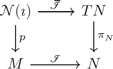
is a vector bundle homomorphism over ℐ, which is fiberwise injective.≫
The notation U|Uα is not described in [5], but by its usage it should be equivalent to U∩p−1(Uα). Note also that, later on, the paper adds the superscript ℐ to Uα and will write it as .
Consider planar immersed curves c : S1⟶ℝ2: normal vectors at c(θ) are a one dimensional space tNc (where Nc is the normal vector to the curve c as defined in Definition 12); hence, the fibre of is one dimensional, so a point in the bundle can be represented by a pair θ ∈ S1, t ∈ ℝ, and the map τℐ becomes the map Φ defined in (52) in Proposition 7. Fix a τ > 0, small, as we will discuss later on. We cover S1 by arcs Uα⊆S1 each shorter than ε, and Wα ⊂ Uα subarcs that can be chosen so that they are an open cover; for small ε we can ensure that tubular coordinates can be perused. The open set U will include normal vectors tNc with |t| < ε.
The statement of main Theorem 1.5 in [5] starts as follows.
Here, is a smooth splitting submanifold of Imm (M, N), diffeomorphic to an open neighborhood of 0 in C∞(N(ℐ)). In particular, the space Immf(M, N) is open in C∞(M, N).≫
The proof covers also the case when M is not compact; we will assume that M is compact so that some arguments can be simplified.
The proof goes as follows.
Indeed, we know that is a diffeomorphism onto its image, and that when , by definition of .
The proof then goes on showing that this φ is smooth (we skip details).
The proof continues as follows.
Some conditions must be added to the definition of to make sure that φ is a diffeomorphism; as was done in (159) to define , by adding the condition : this condition is necessary to apply the representation Theorem 4. No similar condition is present in the proof in [5].
The proof afterwards proceeds as follows.
(this is not the same as the defined in (168), but it has the same scope; the latter one is an open neighborhood of 0 in )
This is the second mistake in the proof.
Even if we restrict the open set described in (195) by adding a first order condition, so that the map (197) properly splits , we have not guarantee that all curves in the associated neighborhood are freely immersed. This is shown in Example 9.
This is why, in our proof, we added the condition τ ≤ rc to the definition of .
We have shown that the proof in [5] does not prove the desired result.
Conflicts of Interest
The author declares no conflicts of interest.
Acknowledgments
The author thanks Prof. Kathryn Mann for her help on the properties of Diff+(S1).
Open Research
Data Availability
No data were used to support this study.

