Modeling and Solution of Vehicle Routing Problem with Grey Time Windows and Multiobjective Constraints
Abstract
Purpose. In order to study the impact of grey delivery time uncertainty on customer satisfaction and delivery costs, a vehicle routing problem with grey delivery time windows and multiobjective constraints is defined. Method. The paper first defines the uncertainty of the delivery vehicle’s arrival time to the customer as grey uncertainty and then whitens the grey time windows; at the same time, the customer’s hard time windows is expanded into a soft time windows to measure customer satisfaction when the vehicle arrives. Experiment. In order to verify the validity of the established model, numerical experiments are carried out in two groups based on the Solomon example, and the solution is solved based on the improved quantum evolution algorithm. Analysis. Distribution cost fluctuations and customer satisfaction fluctuations with grey time windows are relatively small; under different satisfaction threshold conditions, the distribution cost is increased gently with the satisfaction threshold. Conclusion. The grey delivery time windows have certain advantages in solving the random travel time vehicle routing problem.
1. Introduction
The logistics industry is a composite service industry that integrates transportation, storage, and information industries. It covers a wide range of fields, absorbs a large number of jobs, and plays a major role in promoting production and stimulating consumption. It is an important part of the national economy. How to effectively reduce logistics costs, improve logistics delivery efficiency, provide customers with differentiated services, and improve customer satisfaction are important management issues facing logistics companies. The vehicle routing problem is the core problem in the optimization of logistics distribution, as well as the key problem of smart logistics. Scholars have carried out extensive research on this problem and have achieved fruitful results.
Vehicle routing problem (VRP) is a classic combinational optimization problem with NP. With the rise of modern logistics industry, it has become a key component of intelligent logistics. Since Dantzig and Ramser [1] put forward and studied this problem in depth, scholars have conducted extensive research on the VRP problem and several important variants of this problem and achieved a lot of results. Many of them are based on the actual logistics distribution of scholars who added more constraints so that the research results can be better applied to the actual production.
In VRP variants’ problems, as vehicle routing problem with time windows and multiobjective constraints (MOCVRPTW) considers the constraints of customer time windows, customer satisfaction, delivery cost, etc., it is more in line with the “customer first” and in line with the production reality of logistics distribution, which has attracted the attention of academia and industry.
In the actual logistics distribution process, it is necessary to consider not only the uncertainty of vehicle travel time in the distribution process but also how to save the distribution cost to the greatest extent on the basis of meeting the personalized needs of customers. In this paper, a multiobjective solution method under the constraints of grey time windows is proposed. In terms of the processing of grey time windows, the estimation method of grey time windows under 95% confidence level is given. In terms of satisfaction and distribution cost control, the fuzzy gradient function of customer satisfaction is introduced to set different satisfaction thresholds according to customer classification, and then, the Pareto solution set of different examples is obtained according to the threshold. In order to verify the solvability of the model, based on Solomon’s example, this paper extends the customer hard time windows into soft time windows and carries out two groups of numerical experiments. The results show that the fluctuation of distribution cost and customer satisfaction with grey time windows is small. Under different satisfaction threshold conditions, the distribution cost is increased significantly with the increase of satisfaction threshold.
This paper expands the scope of random travel time research and provides decision-making reference for logistics companies. However, this research also has some shortcomings. There is no clear method for customer classification, and the method for setting satisfaction thresholds for different customer categories has not been given. This is also the focus of the author′s next research.
The rest of this paper is arranged as follows. After Section 1, related literature will be reviewed in Section 2, and problems are described and modeled in detail in Section 3. Section 4 presents the grey distribution method for generating time windows. Section 5 describes albino customer satisfaction and grey distribution time. Section 6 presents the methods and results of numerical experiment analysis. Finally, the paper makes a summary in Section 7.
2. Literature Review
Scholars generally refer to the problem of uncertain driving time of distribution vehicles as vehicle routing problem with stochastic travel times (VRPSTT). It mainly studies the change of travel time due to traffic condition, road repair, weather, and other factors, and the change of the travel time satisfies some statistical rule of the vehicle routing problem. Laporte et al. [2] established the opportunity constraint and compensation model of the problem. They believed that the punishment for vehicles should be proportional to the length of delay and designed a branch cutting algorithm to solve the problem. Park et al. [3] constructed three different heuristic algorithms to solve this problem based on a modified deterministic VRP solution algorithm. Subsequently, Qiang et al. [4] and Yang et al. [5], respectively, extended and solved the problem on the basis of Laporte research. Zhang et al. [6] defined the uncertainty of travel time as fuzzy travel time, built a mathematical model with fuzzy travel time, and designed a new hybrid genetic algorithm by effectively combining fuzzy logic and fuzzy control method with the genetic algorithm of traditional vehicle routing problem. Li et al. [7] proposed two models of opportunity-constrained programming and stochastic programming with correction for this problem and designed a hybrid algorithm based on tabu search to solve the model. Tao et al. [8] established an opportunity-constrained programming model for random travel time with simultaneous delivery and pickup and designed a decentralized search algorithm solution strategy. Hou et al. [9] also considered the random vehicle routing problem with uncertain demand and uncertain travel time and proposed an improved genetic algorithm with an adaptive mechanism. Tas et al. [10] studied the vehicle routing problem with soft time windows for random travel time and solved the problem based on tabu search algorithm. Li et al. [11] comprehensively considered the total distance and time of vehicles, as well as the equalization of the distance and time of each vehicle, and designed a multiobjective hybrid genetic algorithm combining simulated annealing and genetic algorithm to solve this problem.
In recent years, the rise of e-commerce has led to the vigorous development of the logistics industry, and the research on this issue has maintained a trend of continuous growth. Binart et al. [12] studied this issue with the overall goal of serving the most customers in the shortest time. Miranda and Conceicao [13] focused on the problem that the waiting time after the vehicle arrives at the customer in advance may affect the follow-up distribution arrangement and designed a new method to estimate the time when the vehicle arrives at each customer and the possibility that the vehicle complies with the customer’s time windows. Errico et al. [14] proposed a two-stage strategy for this problem and designed an accurate branch cutting algorithm. Gomez et al. [15] relaxed the hypothesis of random travel time distribution of scholars in this question and designed a new solution strategy that could adapt to different travel time distributions. Wang et al. [16] first classified or divided customers into service areas and then designed two heuristic algorithms by introducing intimacy. Miranda et al. [17] studied the multiobjective random traveling time vehicle routing problem with both cost and service level and constructed the multiobjective memetic algorithm and multiobjective iterative local search algorithm. Jianli et al. [18] abstracted the freight distribution routing problem of railway logistics center into the optimization of the batch distribution vehicle routing problem with random travel time and service time, established a stochastic programming model with correction, and designed the corresponding algorithm to solve the model. Guimarans et al. [19] studied the random travel time vehicle routing problem with two-bit packing and designed the path optimization algorithm with Monte Carlo simulation and bias randomness. In order to study the collection of urban garbage, Markovi et al. [20] established a model of simultaneous delivery with random demand and travel time. Hashemi Doulabi et al. [21] solved the VRPSTT problem with synchronous access and service time based on the branch and bound method. Liu [22] studied the side-sharing services and proposed an arc-based vehicle-based integer linear programming model in space-time-state networks, which is solved by Dantzig–Wolfe decomposition.
3. Problem Description and Modeling
3.1. Problem Description
Taking the distribution network between the distribution center and the customer point as the research object, suppose that the distribution center has some vehicles of the same type with a capacity of Q, and the vehicles provide delivery services for n customers, where customer i (wherei = 1,2, …, n) wants that the delivery service of a certain car is obtained within the time period of [ETi, LTi]. The vehicle departs from each depot, serves several customers in turn, and returns to the original depot after completing the delivery task.
In the actual distribution, due to the uncertainty of traffic and other factors, time tij spent by the vehicle from customer i to customer j is uncertain. Such uncertainty can be estimated at the upper and lower limits according to experience, which conforms to the characteristics of grey number [23]. Since the customer has uncertainty in the extension of expected time, the paper considers that the delivery time is grey uncertain, and the customer’s expected time windows and satisfaction are known in a fuzzy way. Therefore, the paper takes the distribution cost and customer satisfaction as the optimization objectives to carry out modeling and solving and make a reasonable distribution plan.
3.2. Model Assumptions
To facilitate the elaboration and modeling of the problem, this paper makes the following assumptions. (1) All the distribution vehicles have the same models, that is, the load and speed are the same. (2) Determine a number of loops as vehicle driving routes; the total distance of each circuit will not exceed the maximum driving distance of the vehicle; all loops start from the distribution center and return to the vehicle yard; each customer can only be on one loop; each customer on the loop only takes one car’s service. (3) The total weight of the customer’s goods on each line shall not exceed the vehicle load. (4) The time required for vehicles to enter and exit the distribution center is not taken into account. (5) The service time of all customers shall neither be earlier than the earliest service time tolerated by the customer nor exceed the latest service time tolerated by the customer. Each customer shall have the lowest service level, that is, the needs of the vehicle shall reach the customer’s location within the time windows corresponding to the customer’s lowest satisfaction. (6) The driving cost per unit routing is fixed, and the goal is to minimize the sum of distribution costs of all vehicles.
3.3. Mathematical Model
-
Sets:
- (i)
V: node set (customer set and distribution center), V = {0,1,2, …, n} represents the node set of the directed graph, in which 0 represents the distribution center
- (ii)
V0: the customer set, V0 = {1,2, …, n}
- (iii)
K: the vehicle set, K = {1,2, …, k}
-
Parameters:
- (i)
Q: the rated load of the vehicle
- (ii)
cd: the cost of starting a vehicle
- (iii)
ct: the driving cost of a single vehicle per unit distance
- (iv)
dij: Euclidean distance between customer i and j, i, j ∈ V0, i ≠ j
- (v)
d0i: the distance between the distribution center and the customer i, and d0i = di0, i ∈ V0
- (vi)
Di: the total weight of all the goods of the customer i, i ∈ V0
- (vii)
[ETi, LTi]: the expected service time windows of customer i; ETi is the earliest service time expected by the customer and LTi is the latest service time expected by the customer, i ∈ V0
- (viii)
[ET0, LT0]: opening time of the distribution center
- (xi)
EETi: the earliest service time tolerated by the customer i, i ∈ V0
- (x)
ELTi: the latest service time tolerated by the customer i, i ∈ V0
- (xi)
sti: the time required for the vehicle to serve the customer i, i ∈ V0
- (xii)
tij: the time taken by the vehicle from the customer i to j, i, j ∈ V0, i ≠ j
- (xiii)
: the time taken by the vehicle from the customer i to j at a constant speed state, i, j ∈ V0, i ≠ j
- (xiv)
ti: the time the vehicle arrives at the customer i, i ∈ V0
- (xv)
Ui(ti): the satisfaction of customer i at time ti in the car
- (xvi)
λ: the parameters used to weigh dispatch costs against running costs, λ ∈ [0,1]
-
Decision variables:
- (i)
xijk: the driving variable of vehicle k (k ∈ K), and xijk ∈ {0,1}. If the vehicle k travels from point i to point j, then xijk = 1, otherwise xijk = 1.
- (ii)
L0k: the weight of the goods carried by the vehicle k when it leaves the distribution center.
- (iii)
tik: the time when the vehicle k starts to serve the customer i; if the vehicle k does not serve the customer i, then tik = 0, i ∈ V0, k ∈ K.
Different logistics enterprises can change the value of λ according to their own conditions, that is, change the value of (λ/1 − λ). Then, the model is applicable to the minimum priority of vehicles, the minimum priority of total distance, and other problems in between. For example, if the logistics company has enough vehicles and drivers, then the company does not need to care too much about the startup cost of the vehicle. The value of λ can be appropriately reduced, or even λ = 0. At this time, the vehicle optimization goal is the shortest total delivery distance and no longer considers vehicle startup costs. If the logistics company has insufficient delivery vehicles or insufficient drivers, then it is necessary to consider a larger value of λ, then appropriately increase the value of cd, then the minimum number of vehicles used becomes the first optimization goal, and the total delivery distance becomes the second optimize the target.
4. Grey Delivery Time Windows
Under normal circumstances, the time to reach the destination is often different due to road traffic conditions or nonuniform speed of the vehicle, resulting in uncertainty in the time for the vehicle to reach the customer, but the range of arrival time can be estimated from historical data. Therefore, this paper assumes that the delivery time is grey, and the travel budget time equation in [24] generates vehicle delivery grey time. The specific method is as follows.
The time from node i to node j is affected by many independent random factors. According to the central limit theorem, the sum of the superimposed effects of many small independent factors obeys or approximately obeys a normal distribution [18, 25]. It is assumed that the actual arrival time tij obeys a normal distribution, that is, , where represents the variance of the travel time of the vehicle on the road section ij.
5. Customer Satisfaction
5.1. Fuzzify Customer Time Windows
In the delivery process, customer satisfaction is mainly reflected in whether the vehicle can arrive on time. If the vehicle arrives within the customer’s expected time, the customer’s satisfaction is the highest, and the delayed arrival will cause a decrease in customer satisfaction. In order to reflect the customer’s expected time more accurately, combined with time elements and the actual needs of the customer, the customer’s expected time windows is first blurred, and then, the fuzzy gradient function is used to express the customer’s satisfaction. The fuzzification rules refer to the method of Wang et al. [26]; in the paper by Wang, if the time windows is extended too much, such as extending 100 to both sides, the average customer satisfaction will be higher. At this time, the problem is close to the problem of no time windows requirement, and it is not easy to distinguish various routes. If the expansion is too small, such as 30 for each expansion, the satisfaction degree will be too large, and the average satisfaction degree will be too strongly correlated with the time windows. At this time, the problem is close to the hard time windows requirement, and the expected effect is also not achieved.
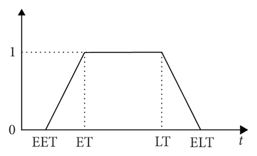
The meaning of equation (18) is that if the customer arrives before the earliest time EET that the customer can tolerate or arrives after the latest time ELT that can be tolerated, the customer is no longer in working hours and cannot deliver the goods, so customer satisfaction is 0. If after the earliest tolerated time EET but before the normal work start time ET or after the normal working time LT but before the latest tolerated time ELT, customer satisfaction can hand over the goods because it is not part of the normal working hours and satisfaction is not high, but the satisfaction level is higher when the arrival time is about close to normal working hours. If the vehicle arrives during normal working hours [ET, LT], the customer is most satisfied with 100% satisfaction (here, marked as 1).
- (1)
If ⊗ti is before the earliest time, the customer can tolerate, which means ⊗ti ≤ EETi; then, the waiting time windows opens, and the customer satisfaction is 0
- (2)
If ⊗ti exceeds the time windows expected by the customer, but is after the earliest tolerable time, ⊗ti ∈ [EETi, ETi), the customer satisfaction value is between [0, 1)
- (3)
If ⊗ti is within the service time windows[ETi, LTi], then the customer satisfaction is 1
- (4)
If ⊗ti exceeds the time windows expected by the customer, but is before the latest tolerable time, ⊗ti ∈ (LTi, ELTi]; then, the customer satisfaction is[0, 1)
- (5)
If ⊗ti exceeds ELTi, which means ⊗ti > ELTi, then the customer satisfaction is 0
5.2. Satisfaction Threshold
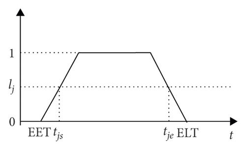
In the actual distribution, the demands of different customer satisfaction are generated according to different products or important levels of customers. In order to save cost and provide personalized service, customers are classified and the minimum satisfaction threshold is set. As shown in Figure 2, for a certain customerj, the minimum satisfaction threshold is lj. Then, corresponding to this threshold, the time interval [tjs, tje] for which the vehicle can serve the customer is the part of the broken line in bold, as shown in Figure 2, which is the part above the line y = lj (including the equal).
5.3. The Matching Problem of Grey Time Windows and Customer Satisfaction Threshold
According to equation (13), under a given confidence level 1-α, the latest time for the vehicle to reach customer i is , so as long as , and the vehicle can decide to depart from customer i to customer j; otherwise, there will be the risk of not being able to deliver even if it reaches customer j.
5.4. Whitening of Grey Delivery Time
Although 5.3 gives the conditions for the selection of the delivery vehicle route, the subsequent calculation requires the time for the vehicle to actually reach the customer j, so the grey number ⊗tij needs to be whitened [27].
- (1)
According to the definition of probability density function, f(x) is the probability density function of random variable x, and the expression is
(19) - (2)
Then, the distribution function F(x) can be obtained:
(20) - (3)
Therefore, as long as the random variable u that obeys [0, 1] is generated, the random whitening value of ⊗tij can be obtained by calculating F−1(u).
5.5. Satisfaction Calculation
- (i)
Step 1: set the satisfaction threshold
- (ii)
Step 2: calculate the number of customers currently served by the vehicle
- (iii)
Step 3: enumerate customers on the current vehicle path
- (1)
Step 3.1: according to (21), calculate the time for the vehicle to leave the current customer and arrive at the next customer
- (2)
Step 3.2: refer to equation (18) and the satisfaction threshold to calculate time tjstart to start serving customer j
- (3)
Step 3.3: bring the service start time calculated in Step 3.2 into equation (18) to calculate the satisfaction of customer j who is receiving service
- (4)
Step 3.4: calculate the departure time according to the equation tjstart + STj, and jump out of the current cycle if all customers to be served by the vehicle are serviced
- (1)
- (iv)
Step 4: calculate the total satisfaction of the current vehicle
6. Experiment and Analysis
In order to solve the model, the author expands the hard time windows into a soft time windows in Solomon’s example and conducts numerical experiments in two groups based on the improved quantum evolution algorithm [28]. A new idea is provided for solving the problem of serious loss of effective information in the quantum evolutionary algorithm by defining the quantum cell body.
There are 3 types of Solomon’s calculation examples: Rdp, Cdp, and Rcdp. The geographic location of customers in the Rdp calculation example meets a random distribution, the geographic location of customers in the Cdp calculation example meets the clustering distribution, and the geographic location of the customer in the Rcdp calculation example is generated by a mixture of random distribution and cluster distribution. Except for the 9 small- and medium-sized customers, the customer size of the remaining 56 examples is 100. Each type of example can be divided into two categories: the first type of vehicle has a short planning time and weak installation capacity. The second type of vehicles has a long planning time and strong installation capacity; among them, Rdp1, Cdp1, and Rcdp1 have a short planning time and a low vehicle loading capacity (both 200), so the customers that each delivery vehicle can serve are relatively limited (about 5–10 customers), while the planning time for Rdp2, Cdp2, and Rcdp2 is longer, the loading capacity of the vehicle is larger (1000, 700, and 1000, respectively), and each delivery vehicle can serve more customers (some routes can exceed 30).
Considering the generality and time economy, take one from the middle position for each small category in the 56 examples of large-scale customers for numerical experiments. The data characteristics of the six calculation examples are shown in Table 1. The table lists the number, number of customers, total number of items, and number of available vehicles for each test case in Solomon’s example.
| Number | Number of customers | Vehicle load | Available vehicles | |
|---|---|---|---|---|
| 1 | C105 | 100 | 200 | 25 |
| 2 | C205 | 100 | 700 | 25 |
| 3 | R105 | 100 | 200 | 25 |
| 4 | R205 | 100 | 1000 | 25 |
| 5 | RC105 | 100 | 200 | 25 |
| 6 | RC205 | 100 | 1000 | 25 |
6.1. Service Quality Analysis under the Constraint of Grey Time Windows
Taking into account that most scholars’ research takes the shortest distance as the optimization goal, in order to facilitate comparison and analysis, in the experiment, this paper also assumes that the vehicle startup cost is 0, and the objective function is λ = 0 in equation (1). The unit journey cost of the vehicle is ct = 1, the quantum evolution algorithm population is 30, and the maximum number of iterations is set to 100.
In order to verify the difference in service quality when the delivery time windows is grey and the delivery time is fixed, 10 experiments were carried out using 6 selected examples. Name the experiment with a grey delivery time windows as Test1, and name the experiment with the vehicle driving at a constant speed, that is, with a fixed delivery time, as Test2. The customer satisfaction and distribution cost information obtained are shown in Table 2.
| Example number | Experiment name | Customer satisfaction | Distribution cost | ||||
|---|---|---|---|---|---|---|---|
| Maximum | Minimum | Variance | Maximum | Minimum | Variance | ||
| C105 | Test1 | 0.98 | 0.97 | 0.0000593 | 369.74 | 363.25 | 9.38 |
| Test2 | 0.98 | 0.90 | 0.0014682 | 372.32 | 363.25 | 18.29 | |
| C205 | Test1 | 0.90 | 0.88 | 0.0000457 | 361.80 | 361.41 | 0.04 |
| Test2 | 0.89 | 0.86 | 0.0001539 | 380.49 | 361.41 | 77.41 | |
| R105 | Test1 | 0.81 | 0.77 | 0.0004081 | 843.32 | 828.81 | 35.54 |
| Test2 | 0.82 | 0.72 | 0.0014266 | 908.23 | 814.62 | 1620.04 | |
| R205 | Test1 | 0.89 | 0.84 | 0.0004327 | 789.13 | 771.72 | 59.07 |
| Test2 | 0.91 | 0.83 | 0.0011436 | 796.22 | 682.84 | 2353.54 | |
| RC105 | Test1 | 0.85 | 0.82 | 0.0001368 | 660.71 | 635.92 | 106.68 |
| Test2 | 0.87 | 0.82 | 0.0000249 | 736.14 | 681.30 | 645.32 | |
| RC205 | Test1 | 0.88 | 0.83 | 0.0004262 | 647.19 | 637.12 | 21.57 |
| Test2 | 0.91 | 0.76 | 0.0038700 | 664.47 | 632.77 | 172.86 | |
As can be seen from Table 2, in terms of customer satisfaction, the average variance of the five calculations for customer satisfaction in Test1 is 0.0002514 and Test2 is 0.001427. In terms of distribution cost, the average variance of the five calculations for the distribution cost in Test1 is 38.71 and that of Test2 is 814.58. The above data shows that, under the grey delivery time windows, the volatility of customer satisfaction and delivery costs is small, and the overall effect of the model is better.
In order to compare the effects of two time processing methods of grey delivery time and random delivery time on vehicle driving distance and customer satisfaction, set α in the study by Qiang et al. [4] to 0.9, and a set of experiments is designed using the above method, named Test3, and the results show that the two methods have no difference in the impact of delivery distance. In terms of customer satisfaction, the variance of customer satisfaction of Test3 is 0.0003673. The results show that the grey time windows method proposed in this paper has certain advantages.
6.2. Experiment and Analysis under Different Satisfaction Thresholds
In order to provide customers with more personalized services while saving business costs, different satisfaction thresholds (the minimum satisfaction of a single customer) can be set for different customers when providing delivery services to customers.
Taking equation (1) as the objective function, without considering the vehicle startup cost, the experimental environment and experimental parameters are the same as 6.1, the customer satisfaction threshold Slim is from 0.1 to 0.9, the step size is 0.1, and the maximum number of iterations for each threshold is set to 100. Calculate the grey distribution time windows, the distribution cost Cf of different threshold constraints, and the average customer satisfaction Sf. The results are shown in Table 3.
| Slim | 0.1 | 0.2 | 0.3 | 0.4 | 0.5 | 0.6 | 0.7 | 0.8 | 0.9 | 1 | |
|---|---|---|---|---|---|---|---|---|---|---|---|
| C105 | Cf | 363.25 | 363.25 | 369.74 | 372.32 | 392.63 | 401.88 | 406.18 | 412.96 | 417.39 | 445.12 |
| Sf | 0.67 | 0.75 | 0.77 | 0.78 | 0.81 | 0.94 | 0.96 | 0.97 | 0.99 | 1.00 | |
| C205 | Cf | 141.54 | 245.98 | 249.35 | 250.15 | 269.00 | 326.52 | 380.49 | 443.23 | 461.85 | 479.11 |
| Sf | 0.42 | 0.62 | 0.63 | 0.69 | 0.77 | 0.80 | 0.84 | 0.87 | 0.90 | 1.00 | |
| R105 | Cf | 609.70 | 646.43 | 654.70 | 692.30 | 727.23 | 750.84 | 796.38 | 800.95 | 814.62 | 905.56 |
| Sf | 0.47 | 0.55 | 0.57 | 0.66 | 0.69 | 0.74 | 0.80 | 0.82 | 0.88 | 1.00 | |
| R205 | Cf | 745.62 | 771.72 | 772.37 | 774.22 | 789.13 | 792.56 | 796.22 | 824.96 | 842.06 | 864.15 |
| Sf | 0.55 | 0.73 | 0.74 | 0.76 | 0.80 | 0.84 | 0.87 | 0.93 | 0.97 | 1.00 | |
| RC105 | Cf | 558.88 | 597.58 | 606.66 | 611.61 | 620.05 | 663.01 | 736.14 | 762.89 | 784.18 | 805.57 |
| Sf | 0.63 | 0.65 | 0.69 | 0.74 | 0.80 | 0.84 | 0.88 | 0.89 | 0.90 | 1.00 | |
| RC205 | Cf | 621.15 | 627.88 | 632.60 | 635.74 | 637.57 | 640.39 | 647.19 | 664.47 | 677.83 | 681.73 |
| Sf | 0.59 | 0.61 | 0.71 | 0.72 | 0.72 | 0.83 | 0.86 | 0.88 | 0.92 | 1.00 |
In order to facilitate understanding and more intuitive performance of the data in Table 3, using Figures 3–8, respectively, the five examples of distribution costs and average under different satisfaction thresholds are shown.
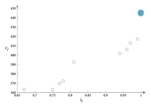
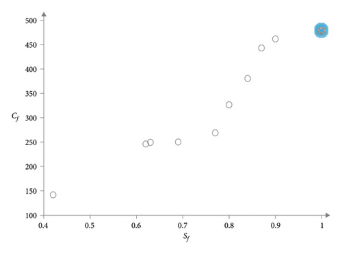
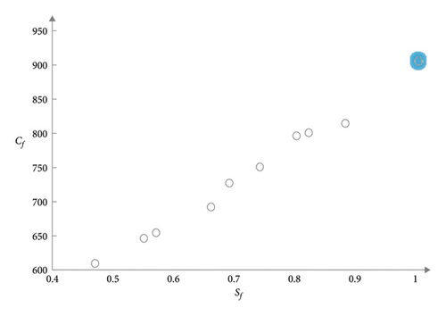
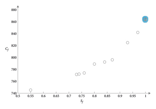
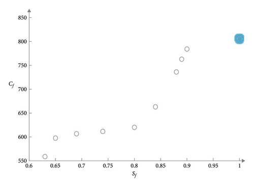
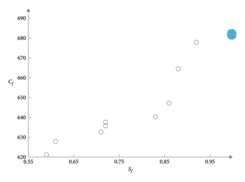
In the six figures, the 10 small circles on the right of each picture correspond to the 10 sets of data in Table 3. The last small blue glowing circle corresponds to the data with a satisfaction degree of 1. When the customer satisfaction threshold is set to 1, it means that the vehicle must arrive within the time windows [ET, LT] expected by the customer. At this time, the problem is transformed into a hard time windows constrained vehicle routing optimization problem (CVRPTW).
This experiment shows that taking into account customer satisfaction, the distribution cost is significantly increased; the distribution cost reaches the highest when the customer satisfaction is 1, that is, under the hard time windows; the distribution cost increases as the satisfaction threshold increases, and the distribution cost gradually increases. In actual production, distribution companies can classify customers and provide personalized distribution services for different customers, so as to achieve the goal of reducing business operating costs without affecting service quality.
In addition, it can be seen from Figures 3 to 8 that the distribution cost gradually increases with the relatively smooth customer satisfaction, indicating that the grey time windows has certain advantages in solving this kind of random travel time vehicle routing problem.
7. Conclusion
The paper abstracts the common problem of uncertain distribution of road conditions into the problem of uncertain distribution time. Combining the grey time windows of delivery with the customer time windows, the choice of vehicle delivery route is decided and customer satisfaction is determined, new grey time windows and multiobjective vehicle routing problem are constructed, and the construction method and whitening of the grey time windows method are given. Finally, based on the improved quantum evolution algorithm, the author designed two sets of numerical experiments on the modified Solomon’s examples. Both sets of experimental results show that the grey time windows has certain advantages in solving the dynamic travel time of the vehicle path and can provide a reference for logistics distribution enterprises.
The grey delivery time windows proposed in this paper expands the research scope of the vehicle routing problem. Since no actual logistics data was used for experiments, this study also has limitations. Simulation experiments based on the operating data of large logistics companies are also the direction of the authors’ future research.
Conflicts of Interest
The authors declare that there are no conflicts of interest regarding the publication of this paper.
Acknowledgments
This research was supported by the following funds: Major Educational and Teaching Reform Research Project of Undergraduate Universities in Fujian Province (FBJG20190284) and Educational and Scientific Research Support Project for Young and Middle-aged Teachers of Fujian Provincial Department of Education (JT180679).
Open Research
Data Availability
The data used to support the findings of this study are available from the corresponding author upon request.


