Assisted Diagnosis of Alzheimer’s Disease Based on Deep Learning and Multimodal Feature Fusion
Abstract
With the development of artificial intelligence technologies, it is possible to use computer to read digital medical images. Because Alzheimer’s disease (AD) has the characteristics of high incidence and high disability, it has attracted the attention of many scholars, and its diagnosis and treatment have gradually become a hot topic. In this paper, a multimodal diagnosis method for AD based on three-dimensional shufflenet (3DShuffleNet) and principal component analysis network (PCANet) is proposed. First, the data on structural magnetic resonance imaging (sMRI) and functional magnetic resonance imaging (fMRI) are preprocessed to remove the influence resulting from the differences in image size and shape of different individuals, head movement, noise, and so on. Then, the original two-dimensional (2D) ShuffleNet is developed three-dimensional (3D), which is more suitable for 3D sMRI data to extract the features. In addition, the PCANet network is applied to the brain function connection analysis, and the features on fMRI data are obtained. Next, kernel canonical correlation analysis (KCCA) is used to fuse the features coming from sMRI and fMRI, respectively. Finally, a good classification effect is obtained through the support vector machines (SVM) method classifier, which proves the feasibility and effectiveness of the proposed method.
1. Introduction
Magnetic resonance imaging (MRI) is a medical imaging technology with rapid development in recent years. It has many advantages such as high contrast for soft tissues, high resolution, and noninvasive way. It is widely used in various types of cardiovascular and cerebrovascular diseases and has promoted the progress and development of contemporary medicine. At present, structural MRI (sMRI) and functional MRI (fMRI) are widely used in the diagnosis of Alzheimer’s disease (AD).
A complete and clear intracranial anatomical structure through hierarchical scanning using sMRI can be obtained, which is helpful to analyze the morphological structure of brain gray matter, white matter, and cerebrospinal fluid and to determine whether a disease or injury exists. The brain structure imaging analysis of patients with AD and normal people (normal control, NC) has found that the gray matter volume of AD patients was significantly lower than that of normal people, and the gray matter in the hippocampus, temporal poles, and temporal islands also has significant shrinkage [1]. Comparing the different stages of AD patients, it is found that hippocampus atrophy is significant in the initial stage. Then, the inferior lateral area of the temporal lobe changes obviously, and finally, the frontal lobe begins to shrink [2]. fMRI is used to measure the changes in hemodynamics caused by neuronal activity which can show the location and extent of brain activation and can detect dynamic changes in the brain over a period of time.
The application of artificial intelligence (AI) in medical treatment has become a research hotspot for scholars at home and abroad [3, 4]. AI combined with machine learning methods is applied to medical image processing to obtain biomarkers and to assist doctors in making correct diagnoses. Deep learning is an important branch of machine learning, and its application in the field of medical imaging has attracted widespread attention. Ehsan Hosseini-Asl [5] and Adrien Payan [6] used 3D convolutional neural networks and autoencoders to capture AD biomarkers. Zhenbing Liu [7] used a multiscale residual neural network to collect multiscale information on a series of image slices and to classify AD, mild cognitive impairment (MCI), and NC. Ciprian D. Billones [8] improved the VGG-16 network for constructing classification model of AD, MCI, and NC. Deep learning algorithms are also widely used in fMRI-assisted diagnosis of brain diseases. Junchao Xiao [9] used stacked automatic encoders and functional connection matrices to classify migraine patients and normal people. Meszlényi Regina [10] proposed a dynamic time normalization distance matrix, Pearson correlation coefficient matrix, warping path distance matrix, and convolutional neural network to realize AD-assisted diagnosis.
With the development of deep learning research, the number of network layers has been continuously deepened. The network structure has gradually become more and more complex, and the requirements for the hardware environment have gradually increased. In order to reduce the environmental demand of the model and to promote the application and improvement of the model, lightweight network operations such as MobileNet [11] and ShuffleNet [12] were born. In this paper, the ShuffleNet model is improved and an AD-assisted diagnosis model based on 3DShuffleNet is proposed, which directly uses the sMRI image preprocessed by the VBM-DARTEL [13] method and uses the deep features of the image to classify AD, MCI, and NC. The proposed method not only reduces the voting link of the slicing method to obtain the test results but also is more conducive to the promotion and application of the model in a low computing power environment because of the use of a lightweight network.
The high-dimensional and small sample characteristics of datasets often bring difficulties of classification and modeling such as fMRI data. Therefore, in this paper, the anatomical automatic labeling (AAL) template is used to calculate the functional link matrix after preprocessing of the original image. Functional connection matrix is a universal and effective method to analyze the correlation characteristics of each brain and can greatly reduce the data dimension. The feature redundancy in the functional connection matrix exists. Thus, data dimensionality reduction and feature extraction are usually improved. Principal component analysis network (PCANet) is an unsupervised deep learning feature extraction algorithm, which can effectively solve the problem of insufficient experimental samples. In this study, PCANet network is used to extract the matrix features and support vector machine (SVM) classifier is used to classify.
In addition, kernel canonical correlation analysis (KCCA) is used to fuse the features of two different modalities to achieve complementary information before the classifier is used, so as to reduce the impact of inherent defects because of a single-modal feature.
2. Data Introduction and Preprocessing
sMRI data are helpful for observing the changes in brain structure during the course of illness. fMRI reflects the influence of illness on brain function by detecting brain activity. The sMRI and fMRI images come from the Alzheimer’s Disease Neuroimaging Initiative (ADNI), and in order to facilitate the fusion of the two modal data information, the experimental data are required to contain both types and the data are obtained at close times. At the same time, because early MCI and late MCI belong to the MCI process and have only slight differences, so they are regarded as the same category. Datasets including 34 cases of AD, 36 cases of MCI (including 18 cases of early MCI, 18 cases of late MCI), and 50 cases of NC were finally selected as experimental data.
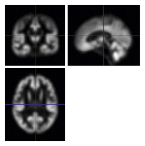
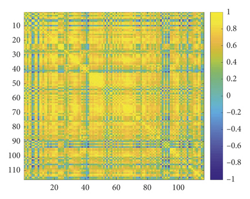
VBM-DARTEL [13] method is used to preprocess sMRI images including segmentation, generating specific templates generation, flow fields generation, and normalization. The above preprocessing steps are all implemented using SPM8 software. Medical image processing software DPABI is used to preprocess fMRI images including the data removal of the first 10 time points, slice timing, realignment, normalization, smoothing, detrending, filtering, and extracting time series to calculate function link matrix. Figure 1(a) shows the coronal, sagittal, and cross-sectional views of gray matter images obtained by sMRI preprocessing, and Figure 1(b) is an example of the functional connection matrix obtained by preprocessing fMRI.
3. Method
The amount of experiment data in this paper is very small; in order to avoid as much as possible the overfitting phenomenon that often occurs in convolutional deep neural networks, this paper uses a lightweight network ShuffleNet with fewer parameters and PCANet that does not require feedback adjustment parameters to implement deep features extraction and classification.
3.1. MRI Feature Extraction and ShuffleNet
ShuffleNet is a deep learning network designed especially for mobile devices with limited computing power. It uses point-by-point grouping convolution and channel shuffling to achieve its high-efficiency architecture [12]. It reduces computational complexity while ensuring that the network still has a good classification performance. The network consists of one convolution layer, one maximum pooling layer, three sets of ShuffleUnit structure, one global pooling layer, and one full connection (FC) layer. Each group of ShuffleUnit structure consists of one ShuffleUnit module like Figure 2(b) and several ShuffleUnit modules like Figure 2(c) connected, and the number of series units is set by the Repeat parameter. ShuffleNet has outstanding performance in image classification [15] and has been applied to face recognition [16]. This network integrates the strengths of many classic networks. It inherits the bottleneck module in the classic deep learning network ResNet [14], as shown in Figure 2(a). It uses the idea of residual learning to speed up model convergence and enhance model performance. It combines MobileNet’s deep capabilities resulting from Separate convolution and AlexNet [17] network grouping method to reduce computational complexity.
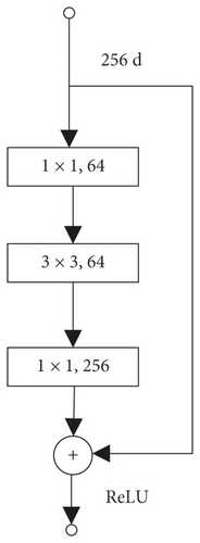
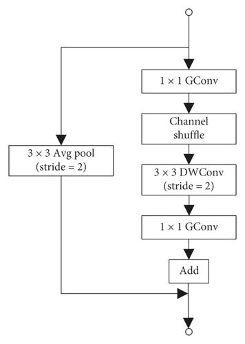
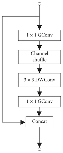
ShuffleUnit is shown in Figure 2, improved from bottleneck in the ResNet network, and the unit output uses the idea of residual learning. The residual learning unit learns the difference between the input layer and the output layer through the parameterized network layer during training process of the network. Reference [16] proves that residual learning is easier to train and classification accuracy of the model is higher than that which directly learns the mapping of input and output. ShuffleUnit not only uses the idea of summation to ensure the transmission of original information to the back layer but also proposes that the first unit in each group of ShuffleUnit uses concat to increase the number of channels and to achieve the purpose of fusion of original information and global information.
Most of the convolutional networks proposed at present are suitable for color images and use 2D convolution to extract image features. In order to adapt to the characteristics of the network, the slicing method is proposed in [5] and [6]. Although the slicing method is convenient for the training and application of existing 2D convolutional neural networks, the result can only represent the category of the corresponding slice of the brain, rather than the overall category. Therefore, the slicing method often requires the majority voting method to integrate the results of each part and further to evaluate the overall category. The process is complicated. In order to avoid the above-mentioned complicated process, the classification features of the entire sample are directly obtained, which facilitates subsequent fusion with fMRI features. Then, a 3D form of ShuffleNet is implemented, and it is also beneficial to retain more three-dimensional spatial information.
In 3DShuffleNet, the number of groups in grouped convolution is set to 3, and in order to adapt to the 3D structure of gray matter images, the 2D convolution is changed to 3D convolution. The parameters of the model structure are shown in Table 1.
| Layer | Ksize | Stride | Repeat | Output (g = 3) |
|---|---|---|---|---|
| Image | 1∗121∗145∗121 | |||
| Conv1 | 3∗3∗3 | 2 | 1 | 24∗61∗73∗61 |
| MaxPool | 3∗3∗3 | 2 | 1 | 24∗31∗37∗31 |
| Stage1 | 2,1 | 1,3 | 240∗16∗19∗16 | |
| Stage2 | 2,1 | 1,7 | 480∗8∗10∗8 | |
| Stage3 | 2,1 | 1,3 | 960∗4∗5∗4 | |
| GlobalPool | 4∗5∗4 | 1 | 960∗1∗1∗1 | |
| FC | 1 | 2 |
Amyloid deposition and neurofibrillary tangles in the brain are typical pathological changes in patients with AD, which can cause brain nerve cell atrophy and death or abnormal signal transmission between cells. Experienced doctors can distinguish AD by observing the degree of atrophy of specific parts of the sMRI imaging. The gray matter of the brain is a dense part of neuronal cell bodies and is the center of information processing. Through it, the distribution and number of neuronal cells in the test patient can be analyzed to screen for AD. In this paper, the sMRI gray matter image obtained after preprocessing is read into this 3DShuffleNet to obtain auxiliary diagnosis results, and the outputs of the penultimate layer and the inputs before the classification layer are regarded as classification features.
3.2. fMRI Feature Extraction
The changes in cerebral hemodynamics over a period of time are recorded in fMRI, so the characteristics of high-dimensional small samples are particularly prominent among them. How to effectively extract the information expressed by brain imaging and reduce the dimensionality has become the primary problem in establishing auxiliary diagnostic models. ALFF value analysis, functional connection matrix analysis, and local consistency analysis are included in the present fMRI data processing methods. Among them, the most common method is functional connection matrix. It measures the coordination and consistency of the work of two brain regions by calculating the Pearson correlation coefficient of the brain interval time series, and it can greatly reduce the data dimension. Because diseases can cause changes in the connection characteristics of certain brain areas, it retains the most AD diagnostic information. In this paper, the functional connection matrix obtained by fMRI preprocessing is used as the input of the auxiliary diagnosis network.
PCANet is a simple deep learning baseline proposed by Chang Tsung-Han [18] which consists of cascaded principal component analysis, binary hash, and block histogram and is widely used in face recognition [19], age evaluation [20], deception detection [21], and other fields. This network has good deep feature extraction capabilities. It can be roughly divided into three stages, among which the first and second stages are PCA convolution, and the third stage is the feature output stage [22].
where l = 1,2, …, L1 and i = 1,2, …, N. The signal ∗ represents two-dimensional convolution.
The third stage is the feature output stage which includes binary hash coding, block histograms for encoding, and downsampling operations.
PCANet is applied to extract effective classification features of AD, and functional connection matrix is calculated as input, using linear SVM classifier to output auxiliary diagnosis results.
3.3. Multimodal Features Fusion Method
sMRI and fMRI images have their own characteristics, which provide information for AD from different angles. The information can be complemented by feature fusion, so as to obtain a more accurate description of samples.
At present, there are few researches on feature fusion in the field of AD-assisted diagnosis and mainly through the concatenation of features to improve the diagnosis effect. In this paper, we take the features extracted from sMRI and fMRI data as the fusion object. Since the images are from the same subject and were obtained on very close dates, it can be considered that there are some certain correlations between the description of the disease in sMRI and fMRI, and the two can be fused by analyzing typical correlation relationship of two feature vectors. At the same time, considering that the correlation is not only linear but also nonlinear, these features from two modal data can be fused by KCCA [23] methods.
CCA [24] is a multivariate statistical analysis method which uses the correlation between the comprehensive variable pairs to reflect the overall correlation between the two sets of indicators. The specific implementation steps are as follows.
Secondly, the second pair of typical variables which are not related to the first pair of typical variables in this group are found, and it is a pair of linear combinations with the second largest correlation.
The process of finding canonical correlation variables is repeated, and the newly found canonical correlation variables are not correlated with the existing ones in the group until all the variables are extracted.
4. Experimental Setup and Model Evaluation
The experimental results in this paper are all obtained under the server equipped with Nvidia TITAN Xp GPU, 32 GB RAM, 256 GB SSD, 2 TB HDD, quad-core Intel Xeon E5-2620 v3 2.4 GHz processor, win10 system, and CUDA10.2 environment configuration. The experimental training set and testing set account for 70% and 30% of the data, respectively.
In sMRI feature extraction and classification experiments, the preprocessed gray matter images are input into the 3DShuffleNet network for training (classification). The model training batch size is set to 4. The Adam optimization algorithm is used. The weight decay value is set to 1e-3, the initial value of the learning rate is set to 1e-3, and it decays exponentially as the number of trainings increases. The total number of iterations is 50, and the attenuation rate is set to 0.9. The 3DShuffleNet model initializes the 3D convolution weights by the normal distribution method. The weights of the BatchNorm3D layer are initialized to a fixed value of 1. The weights of the fully connected layer are initialized to a normal distribution with a mean value of 0 and a variance of 0.001. The bias values are all set to 0. In addition, in order to improve the reliability of the experimental results, the model in this paper and the comparative test model were repeatedly trained and tested for 10 times.
In fMRI feature extraction and classification experiments, by setting different size and number of PCA kernels and block size, the influence on the diagnosis results is explored.
In multimode data fusion experiment, we use the grid search method to adjust KCCA parameters. After that, the classification results of the proposed method in this paper and the experimental dataset in CCA and series fusion method are compared and analyzed.
In order to effectively evaluate the method proposed in this paper, Acc, Sen, Spec, Precision, Recall, F1 score, and AUC are calculated.
5. Experimental Results and Analysis
5.1. Classification Experiments of sMRI
In order to prove the superiority of the 3D model proposed in this paper, some classic models are compared, and the results on sMRI data using 3DShuffleNet are shown in Table 2.
| AD versus NC | Acc | Sen | Spec | Precision | Recall | f1-score | AUC |
|---|---|---|---|---|---|---|---|
| ResNet_10 | 80.4 | 77.0 | 82.7 | 74.9 | 77.0 | 75.8 | 80.9 |
| DenseNet_121 | 74.0 | 53.0 | 88.0 | 77.1 | 53.0 | 61.0 | 79.5 |
| 3DShuffleNet | 85.2 | 69.0 | 96.0 | 93.3 | 69.0 | 79.0 | 86.9 |
| AD versus MCI | Acc | Sen | Spec | Precision | Recall | f1-score | AUC |
| ResNet_10 | 77.5 | 77.0 | 78.0 | 78.0 | 77.0 | 77.4 | 86.2 |
| DenseNet_121 | 62.0 | 61.0 | 63.0 | 64.2 | 61.0 | 61.1 | 68.3 |
| 3DShuffleNet | 84.0 | 84.0 | 84.0 | 84.9 | 84.0 | 84.1 | 91.9 |
| MCI versus NC | Acc | Sen | Spec | Precision | Recall | f1-score | AUC |
| ResNet_10 | 64.8 | 38.0 | 82.7 | 61.6 | 38.0 | 45.8 | 65.5 |
| DenseNet_121 | 53.6 | 52.0 | 54.6 | 47.5 | 52.0 | 47.1 | 55.5 |
| 3DShuffleNet | 64.8 | 43.0 | 79.3 | 60.2 | 43.0 | 48.0 | 67.3 |
| EMCI versus LMCI | Acc | Sen | Spec | Precision | Recall | f1-score | AUC |
| ResNet_10 | 54.0 | 56.0 | 52.0 | 53.7 | 56.0 | 54.1 | 65.2 |
| DenseNet_121 | 54.0 | 28.0 | 80.0 | 62.5 | 28.0 | 36.7 | 48.2 |
| 3DShuffleNet | 53.0 | 40.0 | 66.0 | 56.7 | 40.0 | 45.6 | 58.0 |
It is found from Table 2 that the 3DShuffleNet proposed in this paper has significant advantages, and better classification results on AD versus NC and AD versus MCI are achieved. But the classification effect of MCI versus NC is poor. It is speculated that, on the one hand, because MCI is the early stage of the AD patient, the brain gray matter structure has not changed significantly, and the network is difficult to locate the disease characteristics. On the other hand, because the experimental samples are relatively scarce, the model is not fully trained. Similarly, because the difference between LMCI and EMCI is very slight, the result of LMCI versus EMCI is worst.
In addition, the complexity is evaluated with FLOPs and the number of floating-point multiplication adds. For proving the advantages of the 3DShuffleNet proposed in this paper over other networks, the experimental results of the proposed model on FLOPs are compared with those of the 3D forms of ResNet and DenseNet, which are widely used in image classification. 3DShuffleNet needs 0.79 GFLOPS of computational force, which is much smaller than the comparison models including 3DResNet network with 10 layers and 3DDenseNet network with 121 layers, which requires 38.97 and 89.71 GFLOPs. At the same time, the parameters amount of the network is obtained. 3DShuffleNet has 957.72 thousand parameters; 3DResNet with 10 layers and 3DDenseNet with 121 layers, respectively, have 14.36 and 11.24 million parameters. The proposed network has obtained relatively good classification results with a small computational cost.
5.2. Classification Experiments of fMRI
If the AAL template is used to calculate the function connection, a 90∗90 or 116∗116 function connection matrix will be obtained, respectively, using 90 or 116 regions of cerebrum. Therefore two datasets with different sample sizes are obtained. The whole brain function connection matrix is selected as the experimental data, and the effects of three variables on the classification results are analyzed, respectively.
First of all, the impact of different PCA kernel sizes on the experimental results is compared and analyzed. The initial number of PCA kernels is set to L1 = L2 = 8, and the block size to 16. Because the data have unbalanced categories phenomenon, the average value of sensitivity and specificity is used as evaluation criterion. The detailed results are shown in Figure 3.
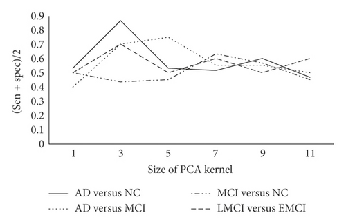
From Figure 3, we can see that, as the PCA kernel’s size continues to increase, the classification result firstly becomes better and then worse. It is speculated that this phenomenon is related to the receptive field theory which is similar to traditional convolutional neural networks. The larger the receptive field is, the more image information can be obtained. So PCANet can obtain better expression ability. However, as the PCA kernel size continues to increase, the number of parameters soars, which reduces the computing efficiency.
Next, the impact of the number of PCA kernels on the classification results is discussed, and the results are shown in Figure 4. Considering that, in different classification combinations, the PCA kernel’s size corresponding to the best classification effect is different, the size of PCA kernel in different classification combinations is set as 3∗3, 5∗5, 7∗7, and 3∗3, and the block size keeps unchanged.
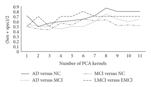
The experimental results show that, in a certain range, the increase in the number of PCA kernels retains more data information as the dimension increases, which makes positioning of the disease more accurate. When the number of PCA kernels reaches a certain level, the experimental result decreases. The reason is that too many PCA kernels will cause the introduction of noise.
Finally, the influence of block size (for histogram calculation) on the robustness of experimental results is analyzed. When the PCA kernel size is set to 3 ∗ 3, 5 ∗ 5, 7 ∗ 7, and 3 ∗ 3 and the number of PCA cores is set to 8, 8, 6, and 6, the experimental results in Figure 5 are obtained.
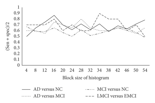
The results show that an appropriate block size provides better robustness, but blindly increasing the block size will sacrifice model performance. After the above-mentioned optimization method of control variables, the experimental results are shown in Table 3.
| Class | Model | Acc | Sen | Spec | Precision | Recall | f1-score | AUC |
|---|---|---|---|---|---|---|---|---|
| AD versus NC | Global brain | 88.0 | 80.0 | 93.3 | 88.9 | 80.0 | 84.2 | 88.7 |
| AD versus MCI | Global brain | 80.0 | 70.0 | 90.0 | 87.5 | 70.0 | 77.8 | 76.0 |
| MCI versus NC | Global brain | 68.0 | 60.0 | 73.3 | 60.0 | 60.0 | 60.0 | 66.7 |
| LMCI versus EMCI | Global brain | 90.0 | 80.0 | 100.0 | 100.0 | 80.0 | 88.9 | 96.0 |
Considering that the size of the PCA kernel, the number of the PCA convolution kernels, and the block size of calculation histogram may affect each other, the grid search method is used for further experiments. The gradient of PCA kernel size is set as [3, 5, 7,…,11], and the gradient of the number of PCA kernels is [1, 2,…,11]. The side length of the block of histogram is set to a multiple of 4, and the maximum value is set to half of the side length of the function connection matrix. The experimental results are shown in Table 4.
| Class | Model | Acc | Sen | Spec | Precision | Recall | f1-score | AUC |
|---|---|---|---|---|---|---|---|---|
| AD versus NC | Cerebrum | 84.00 | 80.0 | 86.7 | 80.0 | 80.0 | 80.0 | 86.0 |
| AD versus MCI | Cerebrum | 85.0 | 90.0 | 80.0 | 81.8 | 90.0 | 85.7 | 78.0 |
| MCI versus NC | Cerebrum | 76.0 | 80.0 | 73.3 | 66.7 | 80.0 | 72.7 | 84.0 |
| EMCI versus LMCI | Cerebrum | 100.0 | 100.0 | 100.0 | 100.0 | 100.0 | 100.0 | 100.0 |
| AD versus NC | Global brain | 88.0 | 80.0 | 93.3 | 88.9 | 80.0 | 84.2 | 88.7 |
| AD versus MCI | Global brain | 85.0 | 90.0 | 80.0 | 81.8 | 90.0 | 85.7 | 87.0 |
| MCI versus NC | Global brain | 80.0 | 80.0 | 80.0 | 72.7 | 80.0 | 76.2 | 83.3 |
| EMCI versus LMCI | Global brain | 100.0 | 100.0 | 100.0 | 100.0 | 100.0 | 100.0 | 100.0 |
The control variable method and the grid search method are used to adjust the parameters, and the global brain function connection matrix is used as the experimental data. It can be seen from Tables 3 and 4 that the grid search method is better than the control variable method in adjusting the parameters, because there is a close relationship between the three variables and they influence each other.
The experimental results obtained from the global brain and cerebrum function connection matrix are compared and analyzed. In general, better performance can be obtained using the whole brain function connection matrix as an experimental sample. Among them, the classification accuracy of AD versus NC and MCI versus NC both increased by 4%, and the classification accuracy of AD versus MCI was equal. The presumed reason is that although AD focuses on appears in the part of cerebrum when one brain area is affected and the other brain areas are intact, the connection characteristics will also change. Therefore, by adding the cerebellum part to enrich the features information, a better diagnosis result can be obtained. In addition to the above results, we also apply our method to classify EMCI and LMCI. It can be seen from the results that the PCANet network is sensitive to the disease progresses from EMCI to LMCI, and functional characteristics changes in brain can be observed, which proves the feasibility and effectiveness of feature extraction using PCANet.
5.3. Classification Experiments of Feature Fusion
In this paper, the z-score standardization method is selected to normalize the features of the two modalities to the same scale, the KCCA feature fusion algorithm is selected to obtain the fused features of sMRI and fMRI, and SVM classifier is used for training and recognition.
In order to prove the effectiveness of the KCCA fusion algorithm, in addition to comparing the difference between the single-modal feature and the fusion feature classification effect, at the same time, the experimental results obtained by using CCA and the series method are compared. In the SVM classifier, the sigmoid kernel is used to train and obtain the recognition results. The experimental results are shown in Table 5. The sMRI features extracted by the 3DShuffleNet network are fused with the fMRI features extracted by the PCANet.
| AD versus NC | Acc | Sen | Spec | Precision | Recall | f1-score | AUC |
|---|---|---|---|---|---|---|---|
| sMRI | 88.0 | 70.0 | 100.0 | 100.0 | 70.0 | 82.4 | 86.0 |
| fMRI | 88.0 | 80.0 | 93.3 | 88.9 | 80.0 | 84.2 | 88.7 |
| CCA | 84.0 | 80.0 | 86.7 | 80.0 | 80.0 | 80.0 | 88.0 |
| Series fusion | 88.0 | 80.0 | 93.3 | 88.9 | 80.0 | 84.2 | 90.0 |
| KCCA | 96.0 | 100.0 | 93.3 | 90.9 | 100.0 | 95.2 | 99.3 |
| AD versus MCI | Acc | Sen | Spec | Precision | Recall | f1-score | AUC |
| sMRI | 90.0 | 90.0 | 90.0 | 90.0 | 90.0 | 90.0 | 97.5 |
| fMRI | 85.0 | 90.0 | 80.0 | 81.8 | 90.0 | 85.7 | 87.0 |
| CCA | 100.0 | 100.0 | 100.0 | 100.0 | 100.0 | 100.0 | 100.0 |
| Series fusion | 90.0 | 90.0 | 90.0 | 90.0 | 90.0 | 90.0 | 98.0 |
| KCCA | 100.0 | 100.0 | 100.0 | 100.0 | 100.0 | 100.0 | 100.0 |
| MCI versus NC | Acc | Sen | Spec | Precision | Recall | f1-score | AUC |
| sMRI | 76.0 | 50.0 | 93.3 | 83.3 | 50.0 | 62.5 | 63.3 |
| fMRI | 80.0 | 80.0 | 80.0 | 72.7 | 80.0 | 76.2 | 83.3 |
| CCA | 76.0 | 50.0 | 93.3 | 83.3 | 50.0 | 62.5 | 69.33 |
| Series fusion | 76.0 | 50.0 | 93.3 | 83.3 | 50.0 | 62.5 | 64.0 |
| KCCA | 100.0 | 100.0 | 100.0 | 100.0 | 100.0 | 100.0 | 100.0 |
| LMCI versus EMCI | Acc | Sen | Spec | Precision | Recall | f1-score | AUC |
| sMRI | 70.0 | 40.0 | 100.0 | 100.0 | 40.0 | 57.1 | 64.0 |
| fMRI | 100.0 | 100.0 | 100.0 | 100.0 | 100.0 | 100.0 | 100.0 |
| CCA | 100.0 | 100.0 | 100.0 | 100.0 | 100.0 | 100.0 | 100.0 |
| Series fusion | 80.0 | 80.0 | 80.0 | 80.0 | 80.0 | 80.0 | 72.0 |
| KCCA | 100.0 | 100.0 | 100.0 | 100.0 | 100.0 | 100.0 | 100.0 |
It can be seen from Table 5 that, compared with the CCA fusion method, the KCCA with rbf kernel has a significant improvement on the recognition results, and by this way, information complementary of two modal is realized. The KCCA algorithm considers the influence of nonlinear features during feature fusion, which makes the feature description more reasonable and enhances the identification ability of subsequent classifiers. This also explains why the effect of feature fusion using CCA is not satisfactory. Compared with the traditional serial fusion method, the KCCA fusion algorithm still has advantages in experiments.
6. Conclusions
Using deep learning algorithms to assist doctors in diagnosing AD has broad research prospects. Furthermore, the idea of features fusion can achieve an obvious improvement. In this paper, 3DShuffleNet is used to build an sMRI-assisted diagnosis model, and PCANet is used to build an fMRI-assisted diagnosis model. Both methods can achieve better results and can provide help on correct diagnosis and early detection of AD. At the same time, the features fusion of two kinds of data is realized, and compared with single modality, better classification results on multiple modalities are obtained. The addition of fMRI features not only further improves the diagnostic advantages of the sMRI-assisted diagnosis model on AD versus NC and AD versus MCI but also avoids the disadvantages of sMRI on the MCI versus NC and LMCI versus EMCI experiments. In addition, multiple modalities methods overcome the shortcomings of single-modal recognition which cannot make full use of target features. The method proposed in this paper also has the characteristics of low requirements for equipment computing capabilities, which is helpful for its promotion in practical applications.
Conflicts of Interest
The authors declare that there are no conflicts of interest regarding the publication of this paper.
Acknowledgments
This work was supported by Joint Project of Beijing Natural Science Foundation and Beijing Municipal Education Commission (no. KZ202110011015) and Natural Science Foundation of China (no. 61671028).
Open Research
Data Availability
The data in this paper come from the Alzheimer’s Disease Neuroimaging Initiative database, which is an open-source third-party database. The specific dataset of the experiment cannot be provided due to copyright reasons. For the experimental data in this paper, subjects who have both fMRI and sMRI are selected. The amount of experimental data is 34 cases of AD, 18 cases of early MCI, 18 cases of late MCI, and 50 cases of NC. ADNI database link: http://adni.loni.usc.edu/.


