In this paper, a double nonmonotone quasi-Newton method is proposed for the nonlinear complementarity problem. By using 3-1 piecewise and 4-1 piecewise nonlinear complementarity functions, the nonlinear complementarity problem is reformulated into a smooth equation. By a double nonmonotone line search, a smooth Broyden-like algorithm is proposed, where a single solution of a smooth equation at each iteration is required with the reduction in the scale of the calculation. Under suitable conditions, the global convergence of the algorithm is proved, and numerical results with some practical applications are given to show the efficiency of the algorithm.

1. Introduction

In this paper, we consider the following nonlinear complementarity problem (NCP): find x ∈ Rⁿ such that

(1)

where F : Rⁿ⟶Rⁿ is continuously differentiable and the superscript T denotes the transpose operator. When F is linear, problem (1) reduces to a linear complementarity problem (LCP). Throughout this paper, the solution set of problem (1), denoted by X^∗, is assumed to be nonempty.

Nonlinear complementarity problems arisen in many practical applications, for example, the KKT systems of mathematical programming problem, the economic equilibrium, the engineering design problem, can be reformulated into the NCP [1–3].

During the past decades, various efficient numerical algorithms are proposed to solve the NCP. One of the most effective methods is to transform the NCP into the semismooth equations (based on nonlinear complementarity function, NCP function) so that the semismooth Newton-type method can be deployed. The most well-known NCP functions are the Fischer–Burmeister function [4] (FB NCP function) and the modified FB NCP function [5]. Sun and Qi [6] proposed several NCP functions, investigated their properties, and provided a numerical comparison between the behavior of different NCP functions. Based on NCP functions, some kinds of algorithm are designed, see, for example, [7–11].

Another well-known class of algorithm is the smoothing algorithm. The main idea of smoothing algorithm is to reformulate the NCP to smooth equations by introducing the smoothing NCP functions. Some smoothing NCP functions and the corresponding algorithms can be found in [12–15].

Besides the NCP functions mentioned above, a 3-1 piecewise NCP function was proposed by Liu et al. [16], using it to solve the inequality-constrained nonlinear optimization. The advantage of the 3-1 piecewise lies in the absence of the smoothing parameter. Motivated by the 3-1 piecewise NCP function, Su and Yang [17, 18] developed smooth-based Newton algorithms with nonmonotone line search for nonlinear complementarity and generalized nonlinear complementarity problems. Different from the previous methods, the authors introduced independent variable quantities to simplify the algorithm, reducing the amount of calculation without using the smoothing parameter.

Smoothing procedure allows one to use successful quasi-Newton approaches, and there are many quasi Newton methods available for the nonlinear complementarity problems based on some smoothing functions [19–26].

In this paper, we will construct a 3-1 piecewise and 4-1 piecewise NCP functions and develop a double nonmonotone quasi Newton method to solve the nonlinear complementarity problems. Based on the piecewise NCP functions, the nonlinear complementarity problem is transformed into the smooth equation. Moreover, we only solve one smooth equation at each iteration. In order to get the better numerical results, a double nonmonotone line search is used by combining with the Broyden-like algorithm. Consequently, the omission of the parameter μ and the single calculation of the Jacobian matrix at each iteration have led to the simplicity and flexibility of this approach. Furthermore, let t = F(x) as an independent variable, which has no relationship with x, ensures the realization of our algorithm easier. Our algorithm is proved to be well-defined and globally convergent under suitable conditions. At the end of the paper, we give numerical results to prove the effectiveness of the algorithm. This paper is organized as follows: the piecewise linear NCP functions are introduced in Section 1. The double nonmonotone line search with quasi-Newton method is given in Section 2. In Section 3, the convergence properties of the algorithm are presented. We give some numerical results in Section 4, and the conclusion is drawn in Section 5.

2. Algorithm Analysis

To describe our algorithm, we first give the definitions of NCP function and P₀ function. We assume that F : Rⁿ⟶Rⁿ is a continuously differentiable P₀-function; if, for all x, y ∈ Rⁿ with x ≠ y, there exists an index i such that

(2)

and we regard a pair (a, b) ∈ R² as an NCP pair if a ≥ 0, b ≥ 0, and a^Tb = 0; a function Φ : R²⟶R is called an NCP function, and we have Φ(a, b) = 0 if and only if (a, b) is a NCP pair.

In what follows, we first introduce the 3–1 piecewise NCP function and then define a 4–1 piecewise NCP function:

(3)

If (a, b) ≠ (0,0), then

(4)

We define the 4–1 piecewise linear NCP function (k is any positive integer):

(5)

If (a, b) ≠ (0,0), then

(6)

where t is a sequence in the algorithm and t = F(x) holds at the optimal solution to NCP.

Hence, the NCP can be written as the following minimization problem:

(7)

To get the solution of (7), we introduce the notations as follows:

(8)

Denote the Jacobian matrix of H(x^k, t^k) by V(x^k, t^k), we get

(9)

The identity matrix of n × n, diagonal matrix whose ith diagonal element is , and the diagonal matrix whose ith diagonal element is are represented by I, , and , respectively.

We use the nonmonotone line search to present Broyden-like method. The search directions d and λ are obtained by calculating a system of smooth equation, and the algorithm is described in detail in Algorithm1.

Algorithm 1:

Step 0: initialization.
Given initial point (x⁰, t⁰) ∈ R²ⁿ, μ ∈ (0,1), ξ > 0, , B₀ = V(x⁰, t⁰), k = 0.
Step 1: if Ψ(x^k, t^k) = 0, then stop. Otherwise, calculate the search direction
. (a)
By (a), we can obtain d^k and λ^k.
Step 2: modified linear search technique.
Step 2.1 If
Ψ(x^k + d^k, t^k + λ^k) ≤ ξΨ(x^k, t^k), (b)
‖Ψ(x^k + d^k, t^k + λ^k)‖ ≤ ξmax_{0≤r≤m(k)−1}‖Ψ(x^k−r, t^k−r)‖, (c)
‖t^k + λ^k − F(x^k + d^k)‖ ≤ ξmax_{0≤r≤m(k)−1}‖t^k−r − F(x^k−r)‖, (d)
where m(0) = 0, 0 ≤ m(k) ≤ min{m(k − 1) + 1, M} is a positive constant. Then, let
x^k+1 = x^k + d^k, t^k+1 = t^k + λ^k, (e)
and go to Step 3; otherwise, go to Step 2.2.
Step 2.2: for j = 0,1, …, check the following inequality with μ^j successively
‖Φ(x^k + μ^jd^k, t^k + μ^jλ^k)‖ ≤ ξmax_{0≤r≤m(k)−1}‖Φ(x^k−r, x^k−r)‖, (f)
‖s^k + μ^jλ^k − F(x^k + μ^jd^k)‖ ≤ ξmax_{0≤r≤m(k)−1}‖t^k−r − F(x^k−r)‖, (g)
Let j_k be the smallest nonnegative integer j such that (f) and (g) hold for μ^j. Set , and
x^k+1 = x^k + ρ_kd^k, t^k+1 = t^k + ρ_kλ^k, (h)
and go to Step 3.
Step 3: Update B_k to get B_k+1,
, (i)
where
. (j)
Select ξ_k to satisfy and matrix B_k+1 is nonsingular.
Step 4: Let k = k + 1, go to Step 1.

3. Convergence Analysis

In this section, the global convergence properties of a Broyden-like algorithm with 3–1 piecewise NCP function are discussed. We give some assumptions to prove the convergence of the algorithm.

Assumption 1.

(a)
Suppose F : Rⁿ⟶Rⁿis P₀-function and it is continuously differentiable.
(b)
On the level set of

(10)

where F is Lipschitz continuously differentiable, namely, there exists a constant Lsuch that for all x₁, x₂ ∈ Rⁿ,

(11)

Remark 1. (see [27]). F(x) is P₀-function, then F ^′(x) is positive semidefinite.

Lemma 1. If H(x⁰, t⁰) ≠ 0, then B₀ = V₀ is nonsingular.

Proof. Assume H(x⁰, t⁰) ≠ 0. If for some (u, v) ∈ R²ⁿ, where and , then

(12)

(13)

By the definitions of and , for all i, and . Therefore, diag(β⁰) is nonsingular. Then

(14)

Substitute v in (12) by (14), and multiply by u^T, we have

(15)

According to the definition of P₀-function, all the principal minor determinants of F′(x) is nonnegative; hence, F′(x) is positive semidefinite. And matrix is positive definite. Therefore u = 0. Together with (14), it holds that v = 0, which implies B₀ is nonsingular.

Lemma 2. Assume that Assumption 1 holds. Then Φ(x^k, t^k)⟶0, as k⟶∞.

Proof. For convenience, we define ‖Φ^l(k)‖ = max_{0≤r≤m(k)−1}‖Φ^k−r‖, where k − m(k) + 1 ≤ l(k) ≤ k. When m(k + 1) ≤ m(k) + 1, we have

(16)

Which means ‖Φ^l(k)‖ is decreasing monotonely, and hence, we have {‖Φ^l(k)‖} convergent. Based on (c) of Algorithm1, we have ‖Φ^l(k)‖ ≤ ‖Φ^{l(l(k) − 1)}‖.

By ξ ∈ (0,1), {‖Φ^l(k)‖}⟶0(k⟶∞) holds, so according to ‖Φ^k+1‖ ≤ ξ‖Φ^l(k)‖⟶0, the conclusion holds.

Lemma 3. Assume Assumption 1 holds. Then t^k − F(x^k)⟶0 as k⟶∞.

Proof. Define ‖t^l(k) − F(x^l(k))‖ = max_{0≤r≤m(k)−1}‖t^k−r − F(x^k−r)‖, where k − M ≤ l(k) ≤ k. For m(k + 1) ≤ m(k) + 1, we have

(17)

From (17), ‖t^l(k) − F(x^l(k))‖ is decreasing in a monotone way; then {‖t^l(k) − F(x^l(k))‖}is convergent.

According to (g) of Algorithm 1, ‖t^l(k) − F(x^l(k))‖ ≤ ξ‖t^{l(l(k) − 10)} − F(x^{l(l(k) − 1)})‖. By ξ ∈ (0,1), {‖t^l(k) − F(x^l(k))‖}⟶0(k⟶∞) holds. That means ‖t^k+1 − F(x^k+1)‖ ≤ ξ‖t^l(k) − F(x^l(k))‖⟶0 holds by Algorithm1, so the conclusion is as follows.

Lemma 4. Assume Assumption 1 holds. Then d^k⟶0, λ^k⟶0, and H^k⟶0, as k⟶∞.

Proof. We have Φ(x^k, t^k)⟶0, [t^k − F(x^k)]⟶0, as k⟶∞ by Lemma 2 and Lemma 3.

So, H(x^k, t^k)⟶0, as k⟶∞:

(18)

We know that B_k is nonsingular by Algorithm1. So, d^k⟶0, and λ^k⟶0, as k⟶∞.

Theorem 1. Under the same condition in Lemma 4, equation (a) of Algorithm1 has solutions, and the definition of Algorithm1 is well.

Proof. On the one hand, we know B₀ is nonsingular by Lemma 1. And B_k produced by the Broyden-like iteration is nonsingular. Hence equation (a) of Algorithm1 has one and only one solution. On the other hand, we know Φ(x^k, t^k)⟶0 and [t^k − F(x^k)]⟶0 as k⟶∞ by Lemma 2 and Lemma 3. So ‖H(x^k, t^k)‖⟶0 as k⟶∞.

Lemma 5. Assume Assumption 1 holds, and let {(x^k, t^k)} be generated sequence by Algorithm1; then {(x^k, t^k)} ⊂ L(x⁰, t⁰).

Proof. By induction, for k = 0, we have (x⁰, t⁰) ∈ L(x⁰, t⁰).

Assume (x^k, t^k) ∈ L(x⁰, t⁰); then we have Ψ(x^k, t^k) ≤ Ψ(x⁰, t⁰). By (c) and (d) of Algorithm1, we get

(19)

So, (x^k+1, t^k+1) ∈ L(x⁰, t⁰). Based on the similar analysis, it is easy to see {(x^k, t^k)} ⊂ L(x⁰, t⁰) for all k.

Theorem 2. Assume Assumption 1 holds, and {(x^k, t^k)} is generated by Algorithm1; then there exists an accumulation point (x^∗, t^∗) of the sequence {(x^k, t^k)} which is solution of NCP(1).

Proof. From Lemma 3 and Lemma 4, we know {(x^k, t^k)} ⊂ L(x⁰, t⁰). By Assumption 1(b), we see that L(x⁰, t⁰) is bounded. So, {(x^k, t^k)} has an accumulation point. Suppose there exists a subsequence which has an accumulation point (x^∗, t^∗). We should prove H(x^∗, t^∗) = 0.

Suppose be an infinite sequence generated by Algorithm1. By construction of the algorithm, we know there are two types of successive iteration. Let K₁ = {k|x^k+1 = x^k + d^k, t^k+1 = t^k + λ^k} and K₂ = {k|x^k+1 = x^k + ρ_kd^k, t^k+1 = t^k + ρ_kλ^k}. We need to prove the conclusion by the following two cases:

Case I: K₁ is an infinite index set. Let the sequence be , which satisfy (b) of Algorithm1. Therefore,

(20)

This suggests that liminf_k⟶∞H(x^k, t^k) = 0.
Case II: K₂ is an infinite index set. Let the sequence be , which satisfy (f) and (g) of Algorithm 1.

It is known that ‖Φ^l(k)‖ is monotone decreasing and lim_k⟶∞‖Φ^k‖ = 0 by Lemma 2 and ‖t^l(k) − F(x^l(k))‖ is monotone decreasing and lim_k⟶∞‖t^k − F(x^k)‖ = 0 by Lemma 3. Therefore, lim_k⟶∞‖H(x^k, t^k)‖ = lim_k⟶∞‖Φ^k‖ + lim_k⟶∞‖t^k − F(x^k)‖ = 0 as k ∈ K₂.

Therefore, the conclusion is followed.

4. Numerical Results

In this section, some numerical results are given. We used a personal computer with 4.0 GB memory and Intel(R) Core(TM)i5-5200U CPU @2.20 GHz to perform all experiments. We used Windows 10 as the operating system and Matlab R2018b to write the computer codes. In the whole experiment, the parameters used in Algorithm1 were ξ = 0.9, μ = 0.8, ξ_k ≡ 1, M is an integer which is randomly selected from 2 to 5. ‖H(x, t)‖ < 10⁻⁶ was the stop criterion.

The number of iterations, the CPU time in seconds, and the value of x^(T)F(x) at the final iteration are are listed in Table 1. x₀ in Table 1 means the Initial point where ones (i, 1) means the i dimension of this problem.

4.1. Some Test Problems

Examples 1–8 (NCP) are considered.

Example 1. Consider (1), where x ∈ Rⁿand F(x) = Mx + q with

(21)

We use x⁰ = (1,1, …,1)^Tand as the starting points to text this problem.

Example 2. Consider (1), where x ∈ R³, and F(x) : R³⟶R³ given by

(22)

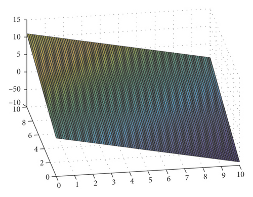
Figure 1 is the 3D diagram of Example 2. (0, λ, 0) is an infinite solution of this problem, where λ ∈ [0,1]. The initial points x⁰, t⁰ are randomly generated, and these elements are in the interval (0,10).

Details are in the caption following the image — **Figure 1**
Open in figure viewer PowerPoint

Diagram of Example 2.

Example 3. Consider (1), where x ∈ R⁷, and F(x) : R⁷⟶R⁷ given by

(23)

Example 4. Consider (1), where x ∈ R⁴ and F(x) : R⁴⟶R⁴ given by

(24)

Example 5. (Kojima–Shindo Problem). Consider (1), where x ∈ R⁴and F(x) : R⁴⟶R⁴ given by

(25)

is a degenerate solution, and (1,0,3,0) is a nondegenerate solution.

Example 6. (Modified Mathiesen Problem). Consider (1), where x ∈ R⁴ and F(x) : R⁴⟶R⁴ given by

(26)

Example 7. The function f(x) is endowed with the component as follows:

(27)

Example 8. Consider (1), where x ∈ Rⁿ and F(x) = Mx + q with

(28)

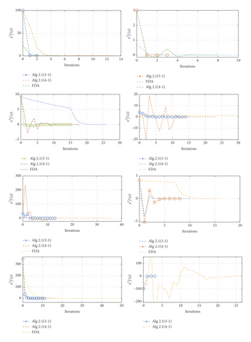
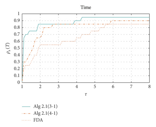
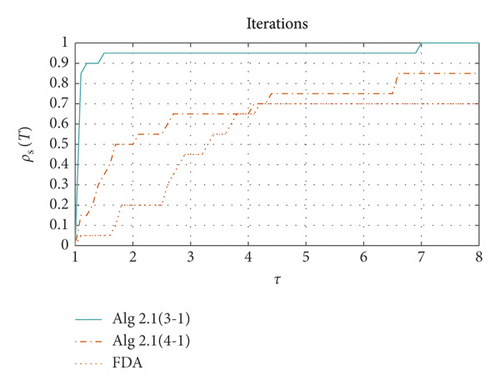
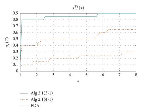
Table 1 shows the results of Examples 1–8 using 3-1 piecewise, 4-1 piecewise Algorithm1 and feasible direction method, respectively. It can be seen from the table that Algorithm1 applying 3-1 piecewise has a good solution to all the above problems. Algorithm1 applying 4-1 piecewise is slightly insufficient, and the feasible direction method has some difficulties in solving examples above, and some of the examples cannot be solved. Figure 2 shows how the x^Tf(x) value of the three algorithms decreases as the number of iterations increases in each specific example. We use performance profiles [28]—distribution functions for a performance metric—as a tool for comparing different algorithms. We consider the comprehensive performance of the above three algorithms in terms of CPU time, number of iterations, and x^Tf(x) value. If the curve is closer to 1, the better the ability to solve the problem (Figure 3).

Table 1. Iterations, CPU time, and x^Tf(x) for NCP Examples 2–6 between Algorithm1 and FDA.

Problem	x⁰	Algorithm 1 with 3–1 piecewise			Algorithm 1 with 4–1 piecewise			Feasible directions algorithm
Problem	x⁰	Iter	CPU time	x^Tf(x)	Iter	CPU time	x^Tf(x)	Iter	CPU time	x^Tf(x)
4.1	ones(100,1)	2	0.000814	5.49E – 09	13	0.001768	1.12E – 08	5	0.004301	6.58E – 07
	ones(100,1)	2	0.473808	5.69E – 08	13	1.520458	1.21E – 08	5	0.257754	−8.81E – 14
	ones(4069,1)	3	15.640096	−1.58E – 11	13	18.551757	1.16E – 08	5	8.556959	7.20E – 14
	ones(8138,1)	2	51.204458	4.51E – 10	13	70.145272	1.44E – 08	5	53.324527	−1.27E – 12
	(1,1,1)^T	3	0.000235	−1.02E – 07	8	0.000617	-5.41E – 08	10	0.000354	4.66E – 07
4.2	(10,10,10)^T	4	0.000288	5.25E – 08	10	0.000604	3.26E – 07	13	0.000529	3.76E – 07
	(1,5,9)^T	7	0.000462	−2.23E – 08	5	0.000742	4.64E – 07	19	0.001465	3.50E – 07
	ones(7,1)	15	0.001014	−2.23E – 08	22	0.001768	5.53E – 07	26	0.004301	6.58E – 07
4.3	10∗ones(7,1)	15	0.001661	−4.62E – 09	24	0.002366	1.05E – 08	NaN	NaN	NaN
4.3	10∗rand(7,1)	16	0.001608	−2.14E – 09	20	0.001204	1.20E – 08	NaN	NaN	NaN
4.4	(1,1,1,1)^T	14	0.007181	−3.11E – 08	23	0.001696	-6.07E – 07	>500∗	Inf	NaN
4.4	(10,10,10,10)^T	145	0.019268	1.80E – 08	86	0.004996	-2.26E – 07	21	0.007137	6.12E – 07
4.5	(1,1,1,1)^T	13	0.00103	−5.62E – 09	26	0.001658	4.93E – 09	36	0.001121	6.43E – 07
4.5	(1,2,3,4)^T	23	0.002497	−5.65E – 07	30	0.003223	-2.75E – 08	65	0.009764	9.61E – 07
4.6	(1,1,1,1)^T	10	0.001351	1.52E – 08	9	0.001473	6.19E – 09	16	0.00746	3.67E – 07
4.7	ones(100,1)	11	0.039089	−9.29E – 11	17	0.001768	8.98E – 08	46	0.024301	8.81E – 07
	ones(1024,1)	20	1.230144	2.26E – 10	20	1.745354	-2.68E – 11	52	1.157443	7.57E – 07
	ones(4069,1)	15	25.532848	−2.61E – 12	20	35.615797	3.61E – 10	55	50.806954	8.14E – 07
	ones(8138,1)	15	305.640096	−4.09E – 14	20	370.126146	4.62E – 09	57	415.720027	7.56E – 07
	ones(100,1)	4	0.002064	7.41E – 07	57	0.107685	1.32E – 07	NaN	NaN	NaN
4.8	ones(1024,1)	6	0.641349	5.40E – 07	407	22.002366	3.10E – 06	NaN	NaN	NaN
	ones(4069,1)	8	26.727794	1.87E – 06	>500^∗	Inf	NaN	NaN	NaN	NaN
	ones(8138,1)	10	215.640096	5.19E – 06	>500^∗	Inf	NaN	NaN	NaN	NaN

4.2. Nash Equilibrium Problem

General economic equilibrium [29] means that total supply and total demand are exactly equal in a price system. With the existing productivity and technical conditions, producers get the most profit, while consumers get the most utility when they meet the budget constraints. The theory of general economic equilibrium was first put forward by the French economist Walras. Walras believes that when the whole economy is in equilibrium, the prices of all consumer goods and factors of production will have a certain equilibrium value, and their output and supply will have a certain equilibrium quantity. It is assumed that the whole economic system is a large and complete trading market, and the equilibrium price system means that all commodities are traded in this market, and finally all commodities can be traded.

Considering the competitive economic model of production and investment, suppose H is a price system, in which there are N kinds of commodities, we use R^N to express commodity space. For producer i, the set of production is Y_i⊆R^N. For consumer j, the set of consumption is Z_j⊆R^N. The number of producers and consumers in the system are l and k, respectively. The total production, total consumption, and initial commodity reserve are represented by Y_i, Z_j, and λ_j, respectively, and the proportion of consumer j in the profit of producer i is represented by ϕ_ji. Specially, i = 1, …, l; j = 1, …, k; and Z_j, Y_i, λ_j ∈ R^N.

To describe the model better, we assume the following definitions. In particular, Z_j, Y_i, and λ_j are independent of x.

Definition 1. Let z_j ∈ Z_j, y_i ∈ Y_i, x is the equilibrium price:

(1)
For every i, the maximum profit function is x · y_i.
(2)
For every j, preference maximum element is .
(3)
Economic equilibrium is defined as .

It can be seen from Definition 1 that when price system H reaches economic equilibrium, the demands of both producers and consumers are satisfied and then all the commodities of price system H are sold, that is, the commodities are cleared. We define the conditions for clearing the goods as

(29)

Equation (29) is not only the equilibrium state of free allocation, but also the model of linear complementarity problem. If Z_j, Y_i, and λ_j are related to x, (29) will become a nonlinear complementarity problem (NCP).

Let the inverse demand function for the market be defined by

(30)

where Q is the total quantity produced, P is the market price, and γ is the elasticity of demand with respect to price. Let q_i denote the output of firm i and let the total cost function for firm i be given by

(31)

Example 9. Data is given in Table 2.

Table 2. Data of Example 9.

Firm i	c_i	L_i	β_i
1	10	5	1.2
2	8	5	1.1
3	6	5	1
4	4	5	0.9
5	2	5	0.8

Example 10. Data is given in Table 3.

Table 3. Data of Example 10.

Firm i	c_i	L_i	β_i
1	5	10	1.20
2	3	10	1.00
3	8	10	0.90
4	5	10	0.60
5	1	10	1.50
6	3	10	1.00
7	7	10	0.70
8	4	10	1.10
9	6	10	0.95
10	3	10	0.75

4.3. Two-Dimensional Contact Problem

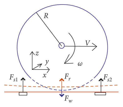
Under the conditions of nonpenetration and negligible attraction between objects, the elastic contact problem mainly requires the contact surface and the pressure of the contact surface when two objects are pressed together. The wheel-rail problem is a typical elastic contact problem.

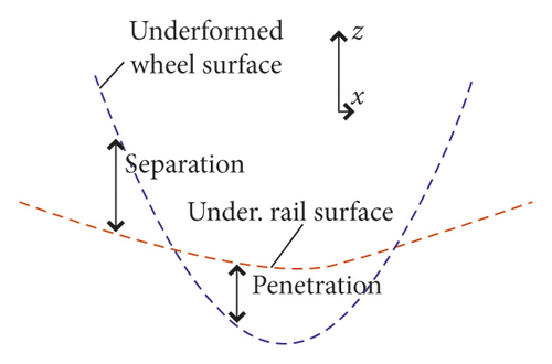
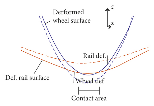
Figure 4 [31] shows the geometric structure application of the wheel-rail contact phenomenon, where Figure 4(a) represents the overall geometric structure showing the forward speed V and angular velocity ω of the track when the wheel is rolling. The track is deformed by the wheel pressure Fw and the sleeper pressure Fs1 and Fs2. At the same time, the wheel deforms due to the wheel-rail pressure Fr, and Figures 4(b) and 4(c) represent the undeformed and deformed states, respectively.

Regarding a point (x, y) on the contact surface, if z represents the pressure on the point, u represents the displacement from the dashed line to the solid line along the normal direction, q represents the distance of the dashed line when the point is not deformed, and w represents its shape, the gap between the rear wheel and the track is w = u + q. Assume that C is the contact surface and E is the other external area, the geometric relationship shown in Figure 4 can be abbreviated as

(32)

If the two-dimensional potential contact area with contact surface is discretized, users mx × my grid is divided, and let n represent the total number of grids; then

(33)

and the problem can be changed into a linear complementarity problem LCP(q, T); to find a pair w, z ∈ Rⁿ, the following is satisfied

(34)

where the coefficient matrix [32] T is a Toeplitz matrix, satisfying

(35)

Example 11. The diagonal element T_k of the coefficient matrix T is

(36)

Example 12. The diagonal element T_k of the coefficient matrix T is

(37)

Example 13. The diagonal element T_k of the coefficient matrix T is

(38)

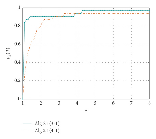
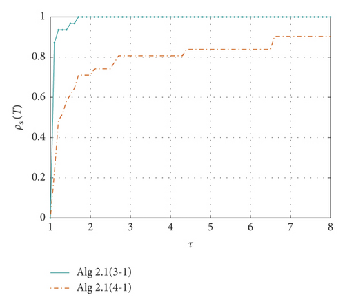
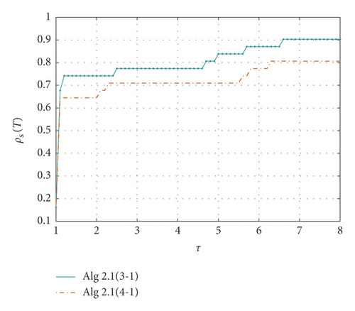
Table 4 shows the performance of Algorithm1 using different piecewise methods for practical application problems. From Figures 5 to 7, it can be seen that Algorithm1 using 3-1 piecewise has a stronger ability to solve all the above problems than Algorithm1 applying 4-1 piecewise.

Table 4. Iterations, CPU time, and x^Tf(x) for problem 4.9–4.13.

Problem	x0	Algorithm 1 with 3–1 piecewise			Algorithm 1 with 4–1 piecewise
Problem	x0	Iter	CPU time	XTF(X)	Iter	CPU time	XTF(X)
4.9	20∗ones(5,1)	20	0.005197	−1.87E − 06	23	0.00523	−1.49E − 06
4.9	30∗ones(5,1)	18	0.010009	−2.28E − 06	21	0.019381	−3.98E − 06
4.10	20∗ones(5,1)	45	0.033759	3.61E − 06	43	0.050365	1.03E − 06
4.10	30∗ones(5,1)	55	0.05047	7.62E − 07	49	0.055852	−1.80E − 06
4.11	ones(100,1)	13	0.052309	1.87E − 08	15	0.089898	1.65E − 08
	ones(1024,1)	14	2.080973	−3.66E − 09	16	2.616348	1.94E − 09
	ones(4069,1)	14	60.367315	1.05E − 09	16	68.659795	8.54E − 09
	ones(8138,1)	14	574.245627	3.05E − 09	20	682.960276	−5.23E − 09
	ones(100,1)	14	0.058579	1.96E − 09	14	0.072436	−5.59E − 09
4.12	ones(1024,1)	14	2.376266	−1.89E − 08	14	2.348159	−4.86E − 09
	ones(4069,1)	12	53.195688	−7.32E − 09	14	61.321038	2.96E − 12
	ones(8138,1)	17	519.846528	−2.89E − 08	14	582.933657	3.25E − 11
	ones(100,1)	17	0.060449	1.99E − 08	19	0.0813907	4.00E − 09
	ones(1024,1)	17	2.860266	5.62E − 08	19	3.145843	8.61E − 09
4.13	ones(4069,1)	17	74.532155	7.27E − 08	19	82.960276	−2.45E − 09
4.13	ones(8138,1)	21	674.226819	2.02E − 08	23	782.155632	5.12E − 09

5. Conclusion

In this paper, by using 3-1 and 4-1 piecewise nonlinear complementarity problem functions, we reformulate the nonlinear complementarity problem into smooth equations. By using a new nonmonotone line search, a modified smooth Broyden-like algorithm is proposed and the global convergence of the proposed algorithm is obtained, and the numerical tests for some practical problems show the efficiency of the algorithm. How to get the local convergence under certain conditions is worth studying in the future.

Conflicts of Interest

The authors declare that there are no conflicts of interests regarding the publication of this paper.

Open Research

Data Availability

The data used to support the findings of this study are included within the article.

References

1 Harker P. T. and Pang J.-S., Finite-dimensional variational inequality and nonlinear complementarity problems: a survey of theory, algorithms and applications, Mathematical Programming. (1990) 48, no. 1–3, 161–220, https://doi.org/10.1007/bf01582255, 2-s2.0-0344704362.
10.1007/BF01582255
Web of Science® Google Scholar
2 Moré J. J., Global methods for nonlinear complementarity problems, Mathematics of Operations Research. (1996) 21, no. 3, 589–614, https://doi.org/10.1287/moor.21.3.589, 2-s2.0-0030204920.
10.1287/moor.21.3.589
Web of Science® Google Scholar
3 Ferris M. C. and Pang J. S., Engineering and economic applications of complementarity problems, Society of Indian Automobile Manufacturers Review. (1997) 39, no. 4, 669–713, https://doi.org/10.1137/s0036144595285963, 2-s2.0-0031352141.
10.1137/s0036144595285963
Google Scholar
4 Fischer A., A special Newton-type optimization method, Optimization. (1992) 24, no. 3-4, 269–284, https://doi.org/10.1080/02331939208843795, 2-s2.0-84948263182.
10.1080/02331939208843795
Google Scholar
5 Chen B., Chen X., and Kanzow C., A penalized Fischer-Burmeister NCP-function, Mathematical Programming. (2000) 88, no. 1, 211–216, https://doi.org/10.1007/pl00011375, 2-s2.0-29244465866.
10.1007/PL00011375
Web of Science® Google Scholar
6 Sun D. and Qi L., On NCP-functions, Computational Optimization and Applications. (1999) 13, no. 1–3, 201–220.
10.1023/A:1008669226453
Web of Science® Google Scholar
7 Luca T., Facchinei F., and Kanzow C., A semismooth equation approach to the solution of nonlinear complementarity problems, Mathematical Programming. (1996) 75, no. 3, 407–439.
10.1007/BF02592192
Web of Science® Google Scholar
8 Jiang H. and Qi L., A new nonsmooth equations approach to nonlinear complementarity problems, SIAM Journal on Control and Optimization. (1997) 35, no. 1, 178193, https://doi.org/10.1137/s0363012994276494, 2-s2.0-0030736633.
10.1137/S0363012994276494
Web of Science® Google Scholar
9 Luca T., Facchinei F., and Kanzow C., A theoretical and numerical comparison of some semismooth algorithms for complementarity problems, Computational Optimization and Applications. (2000) 16, 173–205.
10.1023/A:1008705425484
Web of Science® Google Scholar
10 Qi L. and Yang Y., NCP functions applied to Lagrangian globalization for the nonlinear complementarity problem, Journal of Global Optimization. (2002) 24, 261283.
10.1023/A:1020247804865
Web of Science® Google Scholar
11 Pang J.-S. and Gabriel S. A., NE/SQP: a robust algorithm for the nonlinear complementarity problem, Mathematical Programming. (1993) 60, no. 1–3, 295–337, https://doi.org/10.1007/bf01580617, 2-s2.0-34250083447.
10.1007/BF01580617
Web of Science® Google Scholar
12 Chen C. and Mangasarian O. L., A class of smoothing functions for nonlinear complementarity problems, Journal of Computational and Applied Mathematics. (1997) 80, 105–126.
10.1016/S0377-0427(97)80133-1
Web of Science® Google Scholar
13 Kanzow C. and Pieper H., Jacobian smoothing methods for nonlinear complementarity problems, SIAM Journal on Optimization. (1999) 9, no. 2, 342–373, https://doi.org/10.1137/s1052623497328781, 2-s2.0-0033418367.
10.1137/S1052623497328781
Web of Science® Google Scholar
14 Krejic N. and Rapaji´ c S., Globally convergent Jacobian smoothing inexact´ Newton methods for NCP, Computational Optimization and Applications. (2008) 41, 243–261.
10.1007/s10589-007-9104-2
Web of Science® Google Scholar
15 Qi L. and Li D. H., A smoothing Newton method for nonlinear complementarity problems, Advanced Modeling and Optimization. (2011) 13, no. 2, 141–152.
Google Scholar
16 Liu A., Pu D. G., and Pu D., 3-1 piecewise NCP function for new nonmonotone QP-free infeasible method, Journal of Robotics and Mechatronics. (2014) 26, no. 5, 566–572, https://doi.org/10.20965/jrm.2014.p0566.
10.20965/jrm.2014.p0566
Google Scholar
17 Ke S. and Yang D., A smooth Newton method with 3-1 piecewise NCP function for generalized nonlinear complementarity problem, International Journal of Computer Mathematics. (2018) 95, 1703–1713.
10.1080/00207160.2017.1329531
Web of Science® Google Scholar
18 Ke S. and Yang D., A modified non-monotone method with 3-1 piecewise NCP function for nonlinear complementary problem, Computer Model. New Tech.(2017) 21, no. 1, 47–51.
Google Scholar
19 Qi L. and Sun D., Smoothing functions and smoothing Newton method for complementarity and variational inequality problems, Journal of Optimization Theory and Applications. (2002) 113, no. 1, 121–147, https://doi.org/10.1023/a:1014861331301, 2-s2.0-0036255350.
10.1023/A:1014861331301
Web of Science® Google Scholar
20 Qi L., Sun D., and Zhou G., A new look at Smoothing Newton method for complementarity problems and box constrained variational inequality problems, Antimicrobial resistance. (1997) 97.
Google Scholar
21 Chen X., Qi L., and Sun D., Global and superlinear convergence of the smoothing Newton method and its application to general box constrained variational inequalities, Mathematics of Computation. (1998) 67, no. 222, 519–541, https://doi.org/10.1090/s0025-5718-98-00932-6.
10.1090/S0025-5718-98-00932-6
Web of Science® Google Scholar
22 Tang J., Dong L., Zhou J., and Fang L., A smoothing Newton method for nonlinear complementarity problems, Computational and Applied Mathematics. (2013) 32, no. 1, 107–118, https://doi.org/10.1007/s40314-013-0015-9, 2-s2.0-84879829043.
10.1007/s40314-013-0015-9
Web of Science® Google Scholar
23 Ma C., Chen X., and Tang J., On convergence of a smoothing Broyden-like method for -NCP, Nonlinear Analysis: Real World Applications. (2008) 9, no. 3, 899–911, https://doi.org/10.1016/j.nonrwa.2007.01.008, 2-s2.0-38949101603.
10.1016/j.nonrwa.2007.01.008
Web of Science® Google Scholar
24 Chen B. and Ma C., A new smoothing Broyden-like method for solving nonlinear complementarity problem with a P 0-function, Journal of Global Optimization. (2011) 51, no. 3, 473–495, https://doi.org/10.1007/s10898-010-9640-7, 2-s2.0-80053306622.
10.1007/s10898-010-9640-7
Web of Science® Google Scholar
25 Fan B., A smoothing Broyden-like method with a nonmonotone derivative-free line search for nonlinear complementarity problems, Journal of Computational and Applied Mathematics. (2015) 290, 641–655, https://doi.org/10.1016/j.cam.2015.06.022, 2-s2.0-84936887336.
10.1016/j.cam.2015.06.022
Web of Science® Google Scholar
26 Zheng X. Y., Shi J. R., Yang W., and Yin Q. Y., Nonmonotone smoothing Broyden-like method for generalized nonlinear complementarity problems, Journal of Applied Mathematics and Computing. (2014) 26, 566–572.
Google Scholar
27 Chen J. S. and Pan S. H., A regularization semismooth Newton method based on the generalized fischer-burmeister function for P0 -NCPs, Journal of Computational and Applied Mathematics. (2007) 1, 464–476.
Google Scholar
28 Dolan E. D. and Moré J. J., Benchmarking optimization software with performance profiles, Mathematical Programming. (2002) 91, no. 2, 201–213, https://doi.org/10.1007/s101070100263, 2-s2.0-28244496090.
10.1007/s101070100263
Web of Science® Google Scholar
29 Zhang L.-P. and Zhou Y., A note on economic equilibrium and financial networks, Acta Mathematicae Applicatae Sinica, English Series. (2014) 30, no. 1, 89–98, https://doi.org/10.1007/s10255-014-0272-4, 2-s2.0-84899637647.
10.1007/s10255-014-0272-4
Web of Science® Google Scholar
30 Zhao J., Vollebregt E. A. H., and Oosterlee C. W., A full multigrid method for linear complementarity problems arising from elastic normal contact problems, Mathematical Modelling and Analysis. (2014) 19, no. 2, 216–240, https://doi.org/10.3846/13926292.2014.909899, 2-s2.0-84899739050.
10.3846/13926292.2014.909899
Web of Science® Google Scholar
31 Zhao J., Vollebregt E. A. H., and Oosterlee C. W., A full multigrid method for linear complementarity problems arising from elastic normal contact problems, Mathematical Modelling and Analysis. (2014) 19, no. 2, 216–240, https://doi.org/10.3846/13926292.2014.909899, 2-s2.0-84899739050.
10.3846/13926292.2014.909899
Web of Science® Google Scholar
32 Wu M. H. and Li C. L., A preconditioned modulus-based matrix multisplitting block iteration method for the linear complementarity problems with Toeplitz matrix, Calcolo. (2019) 56, https://doi.org/10.1007/s10092-019-0307-6, 2-s2.0-85064053631.
10.1007/s10092-019-0307-6
Web of Science® Google Scholar

Citing Literature

All articles

A Double Nonmonotone Quasi-Newton Method for Nonlinear Complementarity Problem Based on Piecewise NCP Functions

Abstract

1. Introduction

2. Algorithm Analysis

3. Convergence Analysis