In this paper, a method was proposed based on RBF for numerical solution of first-order differential equations with initial values that are valued by Z-numbers. The proposed method consists of two parts. The first part has stated the amount of limitation of the fragmentation solution, while the second part has described the assurance of the first part. The limitation section also has two parts. The first part has included the initial condition of the problem, while the second part has included the RBF network. The confidence interval was also considered as a function based on the probability function, which has calculated the confidence level of the first part (limitation). The RBF network or the radial-base grid network has three distinct layers: the input layer that is the set of elementary nodes (sensory units); the second layer is the hidden layers with high dimensions, in which the output layer that has responded to the network response and the activation patterns used in the input layer. The advantage of using RBF is that the use of this technique does not require sufficient information. It only relies on the domain and the boundary. In an example, we have showed that our proposed approach could approximate the problem with acceptable confidence.

1. Introduction

The emergence of a new concept of mathematics called fuzzy sets, the study of fuzzy differential equations, provides a suitable basis for mathematical modeling of real-world issues in which there is ambiguity or some uncertainty. For example, in Science and Engineering, many problems are limited to a set of fuzzy differential equations (FDE) through the process of mathematical modeling. As it is not simple to achieve an exact solution, numerical methods should be utilized [1–8]. One of these methods is the radial basis function (RBF) method.

Generally, radial basis functions are methods, which are based on the location method for interpolation of discrete data while have a high convergence rate [9]. This method is one of the most widely used methods for approximating the functions in the theory of modern approximation [10].

RBFs are first used by Broomhead and Lowe [11]. Much of its use is in the theory, design, and applications of RBF networks [12, 13]. In this paper [14], the use of regulation theory for this group of neural networks is presented as a way to enhance the generalization of the new data. In RBF methods, data are interpolated by linear combinations of functions of a function. This method has been very much considered due to high precision and flexibility versus problem geometry, dimensional independence, and ease of implementation. Today, RBFs are used in some cases such as estimation, modeling, prediction, and classification in various fields, including geosciences [15–19]. Besides, these methods are utilized to solve the numerical differential equations with partial derivatives [20]. The main advantage of numerical methods that use RBF is their nonnetwork characteristic. In nonnetworked methods, it is not necessary to produce a regular network in the domain of the problem, which, due to the high computational cost of network production, is the main advantage of these methods to finite difference methods and finite elements, and so on. The geometric feature used in the RBF approximation is the distance between points. The distance in each space dimension is easily calculated, resulting in higher dimensioning and does not increase the complexity of RBF methods. As stated above, a grid-independent grid function does not require a grid and in spite of our data connections between points; only spatial points are used. Thus, several studies have been used based on RBF to solve various equations. For instance, in [21], the radial function of RBF along with the time-dimensional discretization by the BKM boundary node method and the AEM analogue equation method to solve the time-dependent hyperbolic equations in [22] of RBF to solve time-dependent elliptic equations in [23] of RBF along with the MOL lines in the time dimension to solve the time-dependent nonlinear equations in [24] of RBF using the Kansa idea based on Hermitian interpolation for Fokker–Planck equation. In [25], RBF and quasi-spatial methods to solve the sin-Gordon equation are also used in [26] to use the RBF time-independent functions.

As mentioned, the theory of fuzzy sets is a powerful method to model the uncertainties and processing ambiguity and information dependent on mathematical models. But, they need to be trusted to make this information useful. Human beings have a clear capacity to make rational decisions based on obscure, inaccurate, or incomplete information. Formalization of this capacity is at least somewhat difficult to predict. The author proposed a theorem, called a Z-number, which is a regular pair of fuzzy numbers (A, B) [27]. The first component, A is a limitation for values that have an uncertain variable X that has a value or a real value.The second component, B is a measure of reliability for the first component. Typically, A and B are described with natural disadvantages. For example, about 45 minutes, very sure. Yager used Z-number to calculate the waiting time for a bus [28]. Kang Wang used Z-number to make decisions in an ambiguous environment in 2012 [29]. Ezadi and Allahviranloo initially introduced the Z-based generalized neural network and then estimated the Z-based regression [30]. They also presented methods to rank the Z-numbers in 2017 and 2018 [31, 32]. Also, they, in 2019, introduced the Z-Advanced number process [1]. Further investigations have been carried out on Z-numbers by researchers [33–36]. However, a few studies have been conducted in the field of Z-differential equations [37].

In this paper, we try to provide a numerical method to solve the differential equations with an initial value based on Z-numbers. In Section 2, basic concepts and theorems are presented as well. In Section 3, the network of generalized RBF, radial base functions, is introduced. In Section 4, a method for approximating first-order differential equations with a Z value based on the generalized RBF network is presented. In Section 5, numerical examples are presented and ultimately referenced.

2. Preliminaries

This section provides the necessary definitions and required theorems, which are used to propose the model.

Definition 1. (definition of Z-number).

This valuation for Z according to proposal of Zadeh is observed as a restriction in x and is interpreted as follows [27]:

(1)

Indeed, it means that R(y) : y isA⟶Poss(y = u) = μ_A(u).

(2)

where μ_A is the membership function of fuzzy set A and u is a part of y. P_y(u) is the probability density function of y, and P(y = u) is the probability function of y, where as we do not know the basic probability distribution. It is clear from this information that probability distribution function is itself a fuzzy number.

Definition 2. (parametric form of Z-numbers).

Assuming that Z^∗ is set of Z − numbers, an arbitrary Z-number, Z = (A, B) ∈ Z^∗, in the parametric form is represented by an ordered pair of functions:

(3)

and its components satisfy the following requirements:

(4)

Definition 3. (normal Z − numbers).

Let us consider Z to be a Z − numbers, where Z = (A, B). We say that Z is a normal Z-number if h(B) = 1, where h(B) is the height of B [37].

Definition 4. (Z-number initial value problem (ZIVP)).

In real world, most of the phenomena are based on doubt and the information, which we have from various subjects such as economic, political, and physics , which have been evaluated according to verbal valuables. Here, we try to formulate and investigate the mentioned information to the initial value problem, while our initial data are Z-numbers. For instance, evaluate the population growth issue with the Z-number data (population growth, very high, usually) in the starting moment t₀ and consider how is the information in the next time like in t1. For this purpose, first, we consider a ZIVP as (5), and then we study the existence and uniqueness condition of solution of this problem [37]. Assuming that Z^∗ is set of Z-numbers, so, the general form of differential equation initial value based on Z − numbers is defined as follows:

(5)

where t ∈[t₀, T] ⊆ R₊, f is a continuous mapping from [t₀; T] × Z^∗ in to Z^∗, x₀ is a Z-number in Z^∗, and x(t) = (A_x, B_x).

Suppose x^′ is a Z-valuation; then, according to [28],

(6)

where

is a limitation for values and

is a measure of reliability for the first component,

. For

, assuming there is a Hukuhara difference between A_x(t + h) and A_x(t), we define

(7)

where

is the probability distribution function.

2.1. Gaussian Function Definition

The Gaussian function is a function of the form defined as

(8)

where λ, c, and σ are real constant coefficients and e is the Euler number. The shape of this function is symmetric that quickly drops to zero. The constant λ defines the height of the peak of the curve, c determines the location of the center of the peak, and σ is the standard deviation.

3. RBF Networks

The RBF networks , as shown in Figure 1, are of the type of leading networks with an intermediate layer, first introduced by Broomhead and Low [11] (Figure 1). In this method, the transfer function in the intermediate layer of the Gaussian function and in the output layer of the transfer function is linear [38, 39]. Generally, the RBF network training is divided into two parts. The first part is primarily nonmonitoring-type learning. Using clustering methods, the parameters of the basic functions (centers and latitudes) are determined using input information, and in the second part, learning from type is monitored. The weights between the middle and the output layer are determined using slope reduction and linear regression methods. The intermediate neuron of RBF is connected to each of the input neurons with the weight parameters. These parameters are centers of neurons. The output of each intermediate neural is a function of the distance between the input vector X = [x₁, x₂, …, x_n] and the radial center vector r_j = [r_1j, r_2j, …, r_nj], which is calculated as follows:

(9)

The average neuron output can be calculated in different ways. The main transfer function for this aim is the Gaussian function given as follows [39]:

(10)

In this case, λ is a constant coefficient. Finally, outputs of the output layer are calculated from the following equation:

(11)

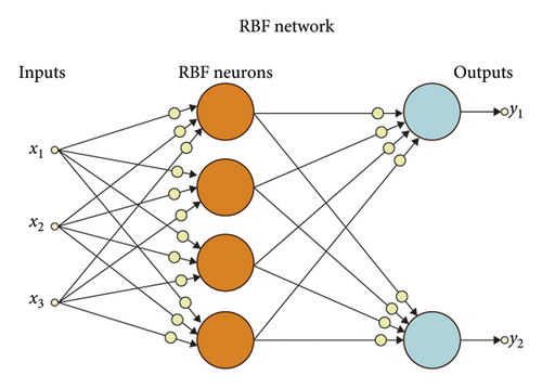
In this regard, w_jk is the weight coefficient between j middle neurons and the k neuron of the output layer and ϕ_j, the output of j is the middle layer neuron. The results of the outcomes were evaluated using root mean square error statistics, RMSE, and determination coefficient R². One of the important points in the RBF network is the choice of the type of transfer function, which is the responsibility of the modeling person. One of the important issues is the attention to the characteristics and statistical variables of the data. For example, if the RBF type is Gaussian, the width of the function is important, which should be chosen so that the distance between the data points is larger, and the dimension of the data is smaller. One of the other issues in designing RBF networks is the number of centers used in the middle layer. As the selection of these centers is directly related to the accuracy and complexity of the network, these centers should be chosen to balance the desired accuracy and complexity.

4. Solving First-Order Differential Equations of Z-Numbers’ Initial Value Using Radial Basic Function (RBF)

Assuming Z^∗ is the set of Z-numbers, the first-order differential equations of Z-numbers’ initial value are defined as follows:

(12)

Equation (12) can be rewritten in the form of the parameter defined in [37]:

(13)

in which in (13),

is a fuzzy function and

is a real function.

and

, respectively, have a certain fuzzy and a real amount,

and

have the role of limitation, and

and

have the role of reliability for [x^′(t)] and

is introduced as follows:

(14)

With the following parametric form,

(15)

where [.]^r is the symbol of r-cut, and

(16)

Theorem 1. ZIVP (12) has a unique Z-process solution.

Proof. Based on [27], relation (12) and relation (13) are equivalent. In (13), is a fuzzy function, and it is introduced on relation (14). For each α-cut, relation (14) and relation (15) are equivalent. On the other hand, the fuzzy initial value problem in (15) has a unique solution (based on Theorem (3.2) in [40]). Similarly . Therefore, it is obvious that ZIVP (12) has a unique solution.

In the general process for obtaining the solution of equation (12) with nonnetworked physical domain methods, we present the problem as a set of scattered points in the domain. These points can be regular or irregular, but they must cover the entire domain in any case. We then approximate the unknown function at any point in the domain. In this way, we consider a base for the solution space and a solution as a linear combination of the base members. In this process, this solution is expanded in terms of base functions. Therefore, the coefficients of the basic sentences are unknown to us. These coefficients must hold in the equations. In the cases where basic radial functions for inwardness are used, the number of centers with the dimension of input data is considered equal in order to achieve high precision. In this paper, we propose a method using the RBF of the generalized RBF-based Z-based numbers in such a way that the initial condition of the main problem is to be established as follows:

(17)

in which,

is a function with a fuzzy value and

can depend on the type of the problem of function with the real or fuzzy value, in which we consider the function with the real value. The values of

and

, respectively, represent the limiting function and the confidence scale for

. With regard to the definition of the Z-number, the interpretation of (17) is described as follows.

If x_T is , then possibility (x_T is ) is .

Here, we define as follows ( is a derivative function):

(18)

which is a method that computes the approximate solution of the equation constraint section, taking into account the initial condition of the problem and is based on the generalized RBF network with fuzzy coefficients. Here, r is the same cut–r that is considered as the center of the RBF network, and ϕ_j(‖t − r_j‖) is defined as follows:

(19)

where φ is a nonlinear function in the space R⁺⟶R, which refers to the transfer function. Some radial base transmission functions φ, in addition to the dependence of the distance function, depend on the factor (ε), which depends on the elongation and extension of the function, whose relation to the standard deviation of the normal distribution (σ) is as follows:

(20)

in which the value of σ² can be determined according to the type of problem. We also utilize the Gaussian radial base transfer function introduced in (15). Some other RBFs with their mathematical relations can be seen in Table 1; r_j are neural network centers, and W is the matrix of the weight coefficients of the output from the intermediate layer to the output layer (w_j). There is a value with fuzzy-value. In fact, when the centers (points) r₁, r₂, …, r_n are constant, the network is trained using the data to find the weight matrix. This process can be done in one form and by data, or by increasing the number of RBF cores, the weight function can be updated in several steps. Training operations begin by dividing the data into training and testing sets. After doing so, the number and position of the RBF centers and the transfer function φ are decided. Training with the implementation of the linear algebra in a system of equations is formed by weights and bias using a pair of input x and each output y.

Table 1. Transition functions used in the radial base function (r = ‖x − r_j‖‖).

Function name	Mathematical relation
Linear	ϕ(r) = r
Cubic	ϕ(r) = \|r\|³
Narrow page	ϕ(r) = r²ln\|r\|
Making	ϕ(r, ε) = (1/1 + εr)
Robey inversion	ϕ(r, ε) = (1/1 + (εr)²)
A few rebates
Multiple reverses

Details are in the caption following the image — **Figure 1**
Open in figure viewer PowerPoint

RBF network diagram.

Moreover,

is a function that specifies the confidence level of the constraint section and is based on the exponential function that we define in terms of the initial condition of the problem in the form as follows:

(21)

Now, with respect to relations (17) and (21), we will have

(22)

has a fuzzy value according to the Z value definition, it can be rewritten in the following form:

(23)

In this case, equation (22) can be rewritten in the following form:

(24)

The value of is also a fuzzy number, which must be computed.

We now want to derive the derivative of the function

i.e.

for this purpose. We derive from the functions of (23), so we have

(25)

In this case,

is calculated as follows:

(26)

To optimize the weights

and

, we use the minimization of the sum-squared error function:

(27)

So, we define it as follows:

(28)

It means that

(29)

4.1. The Numerical Modeling of the Grid Radial Base Function

The RBF algorithm is a function of the distance between the input and some fixed point called center; the function φ is called a radial base function if φ (x) = φ (‖x‖). Therefore, this function φ can be applied to the vector in space Rⁿ but is expressed only in the form of distance. This means that φ can be considered as a numerical function. In these discussions, the application of the Euclidean distance matrix is expressed using the function φ [41]:

(30)

where f (x) is the estimator function, [a₁, …, a_n] are the constant coefficients of the function, and r_i, (i = 1,2, …, n) are the same r-slices. To convert the numerical function φ to the φ matrix, we can use the formulas in the form ϕ(A)_ij = ϕ(A_ij). The function φ is applied to the Euclidean distance matrix and is called the transfer matrix. When the type of transfer function is determined, by using the number n equation, on the input data x(x₁, x₂, …, x_n), we can obtain the coefficients a₁, …, a_n:

(31)

This set holds until vectors x_i ≠ x_j, for i ≠ j and the matrix n × n derived from the set of equations, are inverse. In order to balance the complexity accuracy, we can use all the n data points in this model or that the number of k points, c₁, …, c_k, is considered for the RBF center, which is k ≪ n:

(32)

with assuming the output multiplicity, the generalization function will be given, where α is the vector of coefficients and v is the coefficient matrix. The RBF network, slightly different from the display mode, is a layer of two mappings: first, the mapping space dimensions from Rⁿ n to R^k and then mapped to the output layer R^m [42, 43]:

(33)

where r_j is considered for the RBF center, and in this paper, r_j are cut-r_j and w_jh are output layer weights. In the design of RBF networks, in most cases, the number of central layer units is significantly less than the number of input data, but in the case of interpolation using a radial base function, the number of middle layer centers with dimensions is equivalent to the input data, and its inputs correspond to input data. In the cases where the transfer function is dependent on the variable, for example, the Gaussian function (also depends on the variable σ), and because in many models, it is assumed to be Gaussian (normal), the determination of the width of the function is important. Here, the width factor of the function controls the softness and elongation of the transfer function. When the width of the function is small, the related space and representation of the function are small as well. As a result, a large number of centers are needed for training. In contrast, the estimation accuracy decreases if the space is relevant and represents the broad function. In interpolation methods, it is common practice to use the radial base function to consider the width of all centers.

5. Numerical Examples

In this section, to show the behavior and properties of this new method, we discuss the simulation results of one example. The simulation is conducted on Matlab12, and the objective function in (12) minimizer engaged is fminunc. The initial weights were randomly selected.

Example 1. Consider the following first-order FDE:

(34)

The exact solution of the FDE is

(35)

Assume that the initial value based on Z-numbers is as follows:

(36)

In this case, differential equation (34) can be rewritten as follows:

(37)

And assume that the exact solution of the ZDE is

(38)

Our proposed method is as follows:

(39)

where

(40)

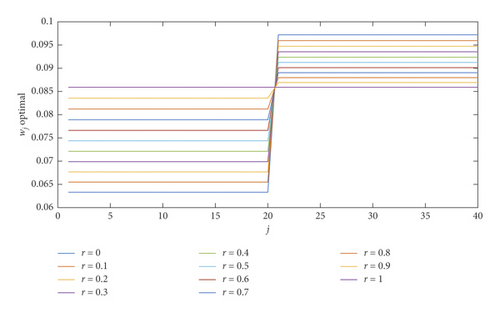
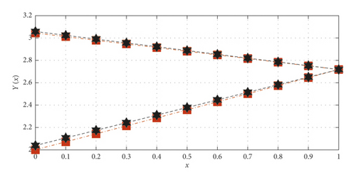
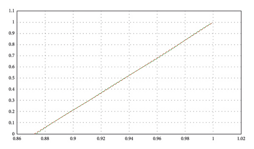
Comparison of the approximate solution with the RBF network training for 50 points and with a choice of λ = 1 is shown in Table 2. The convergence of the neural network weights for each r-cut is shown in Figure 2. Comparison of the approximate method with the exact method is shown in Figure 3. The comparison of the confidence level of the actual answer and the approximate solution is shown in Figure 4.

Table 2. Comparison of the exact Z and Z_T approximated solutions for λ = 1.

r					B_T(t)	B(t)
0	2.00	2.03	3.04	3.05	0.874	0.872
0.1	2.07	2.10	3.02	3.02	0.885	0.885
0.2	2.14	2.17	2.99	2.99	0.899	0.898
0.3	2.21	2.24	2.95	2.95	0.911	0.912
0.4	2.28	2.31	2.92	2.92	0.925	0.925
0.5	2.35	2.37	2.88	2.88	0.937	0.937
0.6	2.42	2.44	2.84	2.85	0.950	0.949
0.7	2.50	2.51	2.81	2.82	0.962	0.962
0.8	2.57	2.58	2.78	2.78	0.975	0.975
0.9	2.64	2.65	2.75	2.75	0.987	0.987
1	2.71	2.71	2.71	2.71	1	1

Example 2. Consider the following first-order ZDE:

(41)

The exact solution of the FDE is

(42)

Assume that the initial value based on Z-numbers is as follows:

(43)

In this case, differential equation (34) can be rewritten as follows:

(44)

And assume that the exact solution of the ZDE is

(45)

Our proposed method is as follows:

(46)

where

(47)

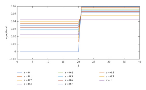
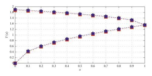
Comparison of the approximate solution with the RBF network training for 50 points and with a choice of λ = 1 is shown in Table 3. The convergence of the neural network weights for each r-cut is shown in Figure 5. The comparison of the approximate method with the exact method is shown in Figure 6. The comparison of the confidence level of the actual answer and the approximate solution is shown in Figure 7.

Table 3. Comparison of the exact Z and Z_T approximated solutions for λ = 1.

r					B_T(t)	B(t)
0	−0.000000002	0	1.87	1.90	0.687	0.663
0.1	0.41	0.42	1.85	1.87	0.769	0.754
0.2	0.58	0.60	1.82	1.84	0.804	0.793
0.3	0.72	074	1.79	1.81	0.833	0.824
0.4	0.83	0.85	1.76	1.78	0.856	0.848
0.5	0.93	0.96	1.72	1.74	0.878	0.873
0.6	1.02	1.05	1.68	1.90	0.899	0.866
0.7	1.11	1.13	1.64	1.65	0.919	0.916
0.8	1.19	1.21	1.58	1.60	0.940	0.937
0.9	1.27	1.28	1.51	1.53	0.963	0.960
1	1.34	1.35	1.34	1.35	1	1

6. Concluding Remarks

In this paper, we proposed a new approach for solving first-order differential equations of Z-numbers’ initial value under uncertainty using radial basic function under generalized H-differentiability. At first, the problem was divided into two parts: the first part of the limitation and the second part of the reliability of the first part. We employed the RBF method for finding upper and lower solutions of the equation of the problem limitation section. The main advantage of this approach is that the fuzzy equation was reduced to the problem of solving two systems of linear equations. Then, we use the information obtained of the proposed method of the first part to calculate the confidence level, and an exponential function was proposed to calculate the reliability of a function. The numerical investigation presented in this paper shows that excellent accuracy can be obtained even when few nodes are used in analysis. In contrast, many more nodes are needed to achieve relatively good accuracy in other methods. Numerical example is included to demonstrate the validity and applicability of the technique and is performed on a computer using a code written in Matlab. The method can be implemented for solving linear and nonlinear equations in higher dimensions.

Conflicts of Interest

The authors declare that they have no conflicts of interest.

Open Research

Data Availability

No data were used to support this study.

References

1 Abbasbandy S. and AllahViranloo T., Numerical solution of fuzzy differential equation by RungeKutta method, Nonlinear Studies. (2004) 11, no. 1, 117–129.
Google Scholar
2 Babolian E., Sadeghi H., and Javadi S., Numerically solution of fuzzy differential equations by Adomian method, Applied Mathematics and Computation. (2004) 149, no. 2, 547–557, https://doi.org/10.1016/s0096-3003(03)00160-7, 2-s2.0-0346279903.
10.1016/S0096-3003(03)00160-7
Web of Science® Google Scholar
3 Chang S. S. L. and Zadeh L. A., On fuzzy mapping and control, IEEE Transactions on Systems, Man, and Cybernetics. (1972) 2, no. 1, 30–34, https://doi.org/10.1109/tsmc.1972.5408553, 2-s2.0-0015285368.
10.1109/TSMC.1972.5408553
Google Scholar
4 Dubois D. and Prade H., Towards fuzzy differential calculus part 3: differentiation, Fuzzy Sets and Systems. (1982) 8, no. 3, 225–233, https://doi.org/10.1016/s0165-0114(82)80001-8, 2-s2.0-0020184062.
10.1016/S0165-0114(82)80001-8
Web of Science® Google Scholar
5 Effati S. and Pakdaman M., Artificial neural network approach for solving fuzzy differential equations, Information Sciences. (2010) 180, no. 8, 1434–1457, https://doi.org/10.1016/j.ins.2009.12.016, 2-s2.0-75149175056.
10.1016/j.ins.2009.12.016
Web of Science® Google Scholar
6 Kaleva O., Fuzzy differential equations, Fuzzy Sets and Systems. (1987) 24, no. 3, 301–317, https://doi.org/10.1016/0165-0114(87)90029-7, 2-s2.0-0023573517.
10.1016/0165-0114(87)90029-7
Web of Science® Google Scholar
7 Puri M. L. and Ralescu D. A., Fuzzy random variables, Journal of Mathematical Analysis and Applications. (1986) 114, no. 2, 409–422, https://doi.org/10.1016/0022-247x(86)90093-4, 2-s2.0-0022674414.
10.1016/0022-247X(86)90093-4
Web of Science® Google Scholar
8 Stefanini L., Sorini L., and Guerra M. L., Parametric representation of fuzzy numbers and application to fuzzy calculus, Fuzzy Sets and Systems. (2006) 157, no. 18, 2423–2455, https://doi.org/10.1016/j.fss.2006.02.002, 2-s2.0-33746823905.
10.1016/j.fss.2006.02.002
Web of Science® Google Scholar
9 Esmaeilbeig M., Paripour M., and Garmanjani G., Approximate solution of the fuzzy fractional Bagley-Torvik equation by the RBF collocation method, Computational Methods for Differential Equations. (2018) 56, 86–214.
Google Scholar
10 Pedrycz W. and Member S., Conditional fuzzy clustering in the design of radial basis function neural networks, IEEE Transactions on Neural Networks. (1998) 9, no. 4, https://doi.org/10.1109/72.701174, 2-s2.0-0032122726.
10.1109/72.701174
PubMed Google Scholar
11 Broomhead D. S. and Lowe D., Multivariable functional interpolation and adaptive networks, Complex Systems. (1988) 2, 321–355.
Google Scholar
12 Moody J. and Darken C. J., Fast learning in networks of locally-tuned processing units, Neural Computation. (1989) 1, no. 2, 281–294, https://doi.org/10.1162/neco.1989.1.2.281.
10.1162/neco.1989.1.2.281
Web of Science® Google Scholar
13 Renals S., Radial basis function network for speech pattern classification, Electronics Letters. (1989) 25, no. 7, 437–439, https://doi.org/10.1049/el:19890300, 2-s2.0-0024622440.
10.1049/el:19890300
Web of Science® Google Scholar
14 Poggio T. and Girosi F., Networks for approximation and learning, Proceedings of the IEEE. (1990) 78, no. 9, 1481–1497, https://doi.org/10.1109/5.58326, 2-s2.0-0025490985.
10.1109/5.58326
Web of Science® Google Scholar
15 Flyer N., Wright G. B., and Fornberg B., Radial basis function-generated fnite differences: a mesh-free method for computational geosciences, Handbook of Geomathematics. (2014) Springer, Berlin, Germany.
Google Scholar
16 Hillier M. J., Schetselaar E. M., de Kemp E. A., and Perron G., Three-dimensional modelling of geological surfaces using generalized interpolation with radial basis functions, Mathematical Geosciences. (2014) 67, 1–23.
Google Scholar
17 Mustafa M. R., Rezaur R. B., Rahardjo H., and Isa M. H., Prediction of pore-water pressure using radial basis function neural network, Engineering Geology. (2012) 135–136, 40–47, https://doi.org/10.1016/j.enggeo.2012.02.008, 2-s2.0-84860283116.
10.1016/j.enggeo.2012.02.008
Web of Science® Google Scholar
18 Ostermann I., Modeling heat transport in deep geothermal systems by radial basis functions, 2011, University of Kaiserslautern, Geomathematics Group, Verlag Dr. Hut GmbH, Munich, Germany, Ph.D. thesis.
Google Scholar
19 Zhang M., Wang K., Zhang C. et al., Using the radial basis function network model to assess rocky desertification in northwest Guangxi, China, Environmental Earth Sciences. (2011) 62, no. 1, 69–76, https://doi.org/10.1007/s12665-010-0498-2, 2-s2.0-79551647968.
10.1007/s12665-010-0498-2
CAS Web of Science® Google Scholar
20 Fornberg B. and Piret C., On choosing a radial basis function and a shape parameter when solving a convective PDE on a sphere, Journal of Computational Physics. (2008) 227, no. 5, 2758–2780, https://doi.org/10.1016/j.jcp.2007.11.016, 2-s2.0-38549128750.
10.1016/j.jcp.2007.11.016
Web of Science® Google Scholar
21 Dehghan M. and Salehi R., A method based on meshless approach for the numerical solution of the two-space dimensional hyperbolic telegraph equation, Mathematical Methods in the Applied Sciences. (2012) 35, no. 10, 1220–1233, https://doi.org/10.1002/mma.2517, 2-s2.0-84862870045.
10.1002/mma.2517
Web of Science® Google Scholar
22 Larsson E. and Fornberg B., A numerical study of some radial basis function based solution methods for elliptic PDEs, Computers & Mathematics with Applications. (2003) 46, no. 5–6, 891–902, https://doi.org/10.1016/s0898-1221(03)90151-9, 2-s2.0-0242667184.
10.1016/S0898-1221(03)90151-9
Web of Science® Google Scholar
23 Uddin M., RBF meshless method of lines for the numerical solution of nonlinear sine-gordon equation, Walailak Journal of Science and Technology (WJST). (2013) 11, no. 4, 349–360.
Google Scholar
24 Kazem S., Rad J. A., and Parand K., Radial basis functions methods for solving Fokker-Planck equation, Engineering Analysis with Boundary Elements. (2012) 36, no. 2, 181–189, https://doi.org/10.1016/j.enganabound.2011.06.012, 2-s2.0-80054799708.
10.1016/j.enganabound.2011.06.012
Web of Science® Google Scholar
25 Mohebbi A., Abbaszadeh M., and Dehghan M., The use of a meshless technique based on collocation and radial basis functions for solving the time fractional nonlinear Schrödinger equation arising in quantum mechanics, Engineering Analysis with Boundary Elements. (2013) 37, no. 2, 475–485, https://doi.org/10.1016/j.enganabound.2012.12.002, 2-s2.0-84872393421.
10.1016/j.enganabound.2012.12.002
Web of Science® Google Scholar
26 Lai S.-J., Wang B.-Z., and Duan Y., Solving Helmholtz equation by meshless radial basis functions method, Progress in Electromagnetics Research B. (2010) 24, 351–367, https://doi.org/10.2528/pierb10062303, 2-s2.0-79959815917.
10.2528/PIERB10062303
Google Scholar
27 Zadeh L. A., A note on Z-numbers, Information Sciences. (2011) 181, no. 14, 2923–2932, https://doi.org/10.1016/j.ins.2011.02.022, 2-s2.0-79955482389.
10.1016/j.ins.2011.02.022
Web of Science® Google Scholar
28 Yager R. R., On Z-valuations using Zadeh’s Z-numbers, International Journal of Intelligent Systems. (2012) 27, no. 3, 259–278, https://doi.org/10.1002/int.21521, 2-s2.0-84857603978.
10.1002/int.21521
Web of Science® Google Scholar
29 Kang B., WEI D., LI Y., and DENG Y., Decision making using Z-numbers under uncertain environment, Journal of Computational Information Systems. (2012) 7, 2807–2814.
Google Scholar
30 Ezadi S. and Allahviranloo N., Numerical solution of linear regression based on Z-numbers by improved neural network, IntellIgent AutomAtIon and Soft ComputIng. (2017) 34, 1–11.
Google Scholar
31 Ezadi S. and Allahviranloo T., New multi-layer method for Z-number ranking using Hyperbolic Tangent function and convex combination, Intelligent Automation Soft Computing. (2017) 24, 1–7.
Web of Science® Google Scholar
32 Ezadi S. and Allahviranloo N., Two new methods for ranking of Z-numbers based on sigmoid function and sign method, International Journal of Intelligent Systems. (2018) 56, 1–12.
Google Scholar
33 Alive R. A., Alizadeh A. V., and Huseynov O. H., The arithmetic of discrete Z-numbers, Information Sciences. (2015) 290, 134–155.
10.1016/j.ins.2014.08.024
Web of Science® Google Scholar
34 Kang B., Wei D., Li Y., and Deng Y., A method of converting Z-number to classical fuzzy number, Journal of Information and Computational Scienc. (2012) 3, 703–709.
Google Scholar
35 Mohamad D., Shaharani S. A., and Kamis N. H., A Z-number based decision making procedure with ranking fuzzy numbers method, AIP Conference Proceedings. (2014) 1635, 160–166.
10.1063/1.4903578
Google Scholar
36 Rafik A. A., Oleg H., Aliyev R., and Alizadeh A., The Arithmetic of Z-Numbers, 2015, World Scientific Publishing Company, Singapore.
Google Scholar
37 Pirmuhammadi S., Allahviranloo T., and Keshavarz M., The parametric form of Z-number and its application in Z-number initial value problem, 2017.
Google Scholar
38 Dibike Y. B., Solomatine D., and Abbott M. B., On the encapsulation of numerical-hydraulic models in artificial neural network, Journal of Hydraulic Research. (1999) 37, no. 2, 147–161, https://doi.org/10.1080/00221689909498303, 2-s2.0-0032650301.
10.1080/00221689909498303
Web of Science® Google Scholar
39 Mason J. C., Price R. K., and Tem’Me A., A neural network model of rainfall-runoff using radial basis functions, Journal of Hydraulic Research. (1996) 34, no. 4, 537–548, https://doi.org/10.1080/00221689609498476, 2-s2.0-0029748915.
10.1080/00221689609498476
Web of Science® Google Scholar
40 Seikkala S., On the fuzzy initial value problem, Fuzzy Sets and Systems. (1987) 24, no. 3, 319–330, https://doi.org/10.1016/0165-0114(87)90030-3, 2-s2.0-0023581045.
10.1016/0165-0114(87)90030-3
Web of Science® Google Scholar
41 Baxter B. J. C., Conditionally positive functions andp-norm distance matrices, Constructive Approximation. (1991) 7, no. 1, 427–440, https://doi.org/10.1007/bf01888167, 2-s2.0-33745879331.
10.1007/BF01888167
Web of Science® Google Scholar
42 Haykin S., Neural Networks: A Comprehensive Foundation, 1999, 2nd edition, Prentice-Hall, New Jersey, NJ, USA.
Google Scholar
43 Zhang A. and Zhang L., RBF neural networks for the prediction of building interference effects, Computers & Structures. (2004) 82, no. 27, 2333–2339, https://doi.org/10.1016/j.compstruc.2004.05.014, 2-s2.0-4944239007.
10.1016/j.compstruc.2004.05.014
Web of Science® Google Scholar

All articles

Solving First-Order Differential Equations of Z-Numbers’ Initial Value Using Radial Basic Function

Abstract

1. Introduction

2. Preliminaries

2.1. Gaussian Function Definition

3. RBF Networks

4. Solving First-Order Differential Equations of Z-Numbers’ Initial Value Using Radial Basic Function (RBF)

4.1. The Numerical Modeling of the Grid Radial Base Function

5. Numerical Examples

6. Concluding Remarks

Conflicts of Interest

Open Research

Data Availability

References

Figures

References

Information

About Wiley Online Library

Help & Support

Opportunities

Connect with Wiley

Solving First-Order Differential Equations of Z-Numbers’ Initial Value Using Radial Basic Function

Abstract

1. Introduction

2. Preliminaries

2.1. Gaussian Function Definition

3. RBF Networks

4. Solving First-Order Differential Equations of Z-Numbers’ Initial Value Using Radial Basic Function (RBF)

4.1. The Numerical Modeling of the Grid Radial Base Function

5. Numerical Examples

6. Concluding Remarks

Conflicts of Interest

Open Research

Data Availability

References

Figures

References

Related

Information