International Journal of Differential Equations

Volume 2020, Issue 1 4325640

Research Article

Open Access

Stability Analysis of a Fractional-Order Model for Abstinence Behavior of Registration on the Electoral Lists

O. Balatif,

Corresponding Author

O. Balatif

[email protected]

orcid.org/0000-0003-1887-5350

Laboratory of Dynamical Systems, Mathematical Engineering Team, Department of Mathematics, Faculty of Sciences El Jadida, Chouaib Doukkali University, El Jadida, Morocco ucd.ac.ma

Search for more papers by this author

L. Boujallal,

L. Boujallal

Department of Mathematics, Faculty of Sciences Ain Chock, University Hassan II, Casablanca, Morocco uh2c.ac.ma

Search for more papers by this author

A. Labzai,

A. Labzai

orcid.org/0000-0002-4417-8893

Laboratory of Analysis, Modeling and Simulation, Department of Mathematics, Computer Science, Faculty of Sciences Ben M’Sik, Hassan II University Mohammedia, Casablanca, Morocco univh2c.ma

Search for more papers by this author

M. Rachik,

M. Rachik

orcid.org/0000-0002-5118-2786

Laboratory of Analysis, Modeling and Simulation, Department of Mathematics, Computer Science, Faculty of Sciences Ben M’Sik, Hassan II University Mohammedia, Casablanca, Morocco univh2c.ma

Search for more papers by this author

O. Balatif,

Corresponding Author

O. Balatif

[email protected]

orcid.org/0000-0003-1887-5350

Laboratory of Dynamical Systems, Mathematical Engineering Team, Department of Mathematics, Faculty of Sciences El Jadida, Chouaib Doukkali University, El Jadida, Morocco ucd.ac.ma

Search for more papers by this author

L. Boujallal,

L. Boujallal

Department of Mathematics, Faculty of Sciences Ain Chock, University Hassan II, Casablanca, Morocco uh2c.ac.ma

Search for more papers by this author

A. Labzai,

A. Labzai

orcid.org/0000-0002-4417-8893

Laboratory of Analysis, Modeling and Simulation, Department of Mathematics, Computer Science, Faculty of Sciences Ben M’Sik, Hassan II University Mohammedia, Casablanca, Morocco univh2c.ma

Search for more papers by this author

M. Rachik,

M. Rachik

orcid.org/0000-0002-5118-2786

Laboratory of Analysis, Modeling and Simulation, Department of Mathematics, Computer Science, Faculty of Sciences Ben M’Sik, Hassan II University Mohammedia, Casablanca, Morocco univh2c.ma

Search for more papers by this author

First published: 22 June 2020

https://doi.org/10.1155/2020/4325640

Citations: 2

Academic Editor: Peiguang Wang

Share a link

Email
Wechat
Bluesky

Abstract

In this work, we propose a fractional-order model that describes the dynamics of citizens who have the right to register on the electoral lists and the negative influence of abstainers on the potential electors. By using Routh–Hurwitz criteria and constructing Lyapunov functions, the local and the global stability of abstaining-free equilibrium and abstaining equilibrium are obtained. Finally, some numerical simulations are performed to verify the theoretical analysis, and they are given for different parameter setting of the order of derivative α.

1. Introduction

The first appearance of the fractional calculus was in a letter written to Guillaume de l’Hôpital by Gottfried Wilhelm Leibniz in 1695 [1–3]. It has become an important field of mathematics due to its immense application in different areas such as chemistry, physics, engineering, psychology, finance, and control theory [4–13, 14].

Mathematical modeling by differential fractional equations has more advantages for modeling and describing the dynamics of memory phenomena that have hereditary properties because fractional derivatives depend not only on local conditions but also on the past and the history of the phenomenon studied. This is, precisely, more suitable and reasonable when modeling sociological phenomena and description of real-world problems.

In this work, we introduce a fractional order for the model developed by Balatif et al. in [15], which describes the dynamics of citizens who have the right to register on the electoral lists and the negative influence of abstainers, who abstain registration on the electoral lists and the electoral process, on the potential electors. The population N is divided into three compartments: the potential electors (P) are entitled to participate in the elections, and they are not yet registered on the electoral lists; the abstainers (A) who have an attitude of abstaining the elections and the registration on the electoral lists; and the registered (R) who are listed on the electoral lists and wish to vote in the elections:

()

where D^αP, D^αA, and D^αR are the derivatives of P(t), A(t), and R(t), respectively, of an arbitrary order α (where

) in the sense of Caputo. Note that when α = 1, the fractional-order model (1) represents the classical PAR model studied in [15]. P(0) ≥ 0, A(0) ≥ 0, and R(0) ≥ 0 are the given initial states.

We note that all parameters are nonnegative. They are defined in Table 1.

Table 1. Parameters description.

Parameter	Definition
Λ	Recruitment rate
β	Effective contact rate
δ	Registration rate of the potential electors on the electoral lists
γ	Registration rate of the abstainers on the electoral lists
μ	Natural mortality rate

There exist several definitions of the fractional derivative operator: Riemann–Liouville, Caputo, Grunwald–Letnikov, etc [16–19]. The reasons to use the Caputo fractional derivative in this work are firstly, the fractional derivative of a constant is zero, and the second reason is that the initial conditions for the fractional-order differential equations with Caputo’s derivatives are in the same form as for the integer-order differential equations [19–21].

This paper is organized as follows. In Section 2, we present some preliminaries about the fractional calculus. In Section 3, we give some basic properties of the model. Section 4 is devoted to analyze the local and global stability of the proposed fractional-order model. Numerical simulations are given and discussed in Section 5. Finally, we conclude the paper in Section 6.

2. Preliminaries

Firstly, we introduce the definition of the Caputo fractional derivative, and we present some functions and useful properties that are used throughout this work [17, 19, 21]:

(1)
The Caputo fractional derivative of order α > 0 of a continuous function f : ℝ₊⟶ℝ is given by

()

where D = d/dt,

, and Γ(.) is the gamma function.

In particular, when

, we have

()

(2)
The Laplace transform of the Caputo fractional derivative is given by

()

with F(λ) the Laplace transform of f(t).

(3)
Let α, β > 0. The Mittag-Leffler function E_α,β of parameters α and β is defined as follows:

()

(4)
The Laplace transform of the Mittag-Leffler functions is

()

(5)
Let α, β > 0 and z ∈ ℂ, then the Mittag-Leffler function satisfies the equality given by

()

(6)
Let f : ℝⁿ⟶ℝⁿ with n ≥ 1. Consider the following fractional-order system:

()

with

, t₀ ∈ ℝ, and x₀ ∈ ℝⁿ. For the global existence of a solution of system (9), we need the following lemma.

Lemma 1 (see [22].)Assume that f satisfies the following conditions:

(i)
f(x) and (∂f/∂x)(x) are continuous for all x ∈ ℝⁿ
(ii)
‖f(x)‖ ≤ ω + λ‖x‖ for all x ∈ ℝⁿ, where ω and λ are the two positive constants

Then, system (9) has a unique solution on [t₀, +∞).

3. Basic Properties of the Model

System (1) describes human population, and therefore it is necessary to prove that all solutions of system (1) with positive initial data will remain positive for all times t > 0 and are bounded. This will be established by the following lemma and theorems.

Lemma 2. The feasible region Ω defined by

()

with initial conditions P(0) ≥ 0, A(0) ≥ 0, and R(0) ≥ 0, is a positive invariant for system (1), where N(0) represents the initial values of the total population.

Proof. The fractional derivative of the total population, obtained by adding all the equations of model (1), is given by

()

Applying the Laplace transform in the previous inequality, we obtain

()

then

()

from (6), we deduce

()

using (7), we have

()

since

()

therefore,

()

It implies that the region Ω is a positive invariant set for system (1).

Theorem 3. The fractional-order initial value problem (1) has a unique solution.

Proof. Let

()

where F is the right side of system (1).

Firstly, it is easy to see that F(X) and (∂F/∂X)(X) satisfy the first condition of Lemma 1.

Secondly, system (1) can be rewritten as follows:

()

where

()

Since

()

where

()

Then, system (1) has a unique solution on [0, +∞).

Theorem 4. If P(0) ≥ 0, A(0) ≥ 0, and R(0) ≥ 0, then the solutions P(t), A(t), and R(t) of system (1) are positive for all t ≥ 0.

Proof. It follows from the first equation of system (1) that

()

Since A(t) is bounded by a constant Λ₀, we have

()

where c is a constant equal to β(Λ₀/N) + (δ + μ).

Applying the Laplace transform in the previous inequality, we obtain

()

from (6), we deduce

()

then

()

Since E_α,1(−ct^α) ≥ 0, therefore the solution P(t) is positive.

Similarly, from the second and third equations of (1), we can easily prove that A(t) and R(t) are positive for all t ≥ 0.

4. Stability Analysis

In this section, we will study the stability behavior of system (1) at an abstaining-free equilibrium point and an abstaining equilibrium point. System (1) has two equilibrium points:

(i)
Abstaining-free equilibrium given by E⁰ = ((Λ/δ + μ), 0, (αΛ/μ(δ + μ))).

This equilibrium corresponds to the case when there are no abstainers in the population.

(ii)
Abstaining equilibrium point, if ℜ₀≻1, given by E^∗ = (P^∗, A^∗, R^∗), where P^∗ = (Λ(γ + μ)/μβ), A^∗ = ((Λ(δ + μ)(ℜ₀ − 1))/μβ), and R^∗ = ((δΛ²(γ + μ)² + γΛ(δ + μ)(γ + μ)(ℜ₀ − 1))/μβ(γ + μ)).

This equilibrium corresponds to the case when the behavior of abstaining the registration on the electoral lists is able to invade the population.

Where ℜ₀ is the basic reproduction number given by

()

In epidemiology, the basic reproduction number ℜ₀ is defined as the average number of secondary infections produced by an infected individual in a completely susceptible population.

In the context of our work, this threshold indicates the average number of persons that an abstainer will “infect” during his “infection” period within the potential elector population, so that the infected individuals will enter to the compartment of abstainers. This number can be obtained by using the next-generation matrix method formulated in [15, 23, 24].

4.1. Local Stability Analysis

In this section, we analyze the local stability of the abstaining-free equilibrium and the abstaining equilibrium.

Theorem 5. The abstaining-free equilibrium E⁰ is locally asymptotically stable if ℜ₀ < 1, whereas E⁰ is unstable if ℜ₀ > 1.

Proof. The Jacobian matrix at E⁰ is given by

()

Therefore, eigenvalues of the characteristic equation of are

()

Therefore, all the eigenvalues of the characteristic equation are negative if ℜ₀ < 1. Thus, |arg(λ_i)| = π≻(απ/2) for i = 1,2,3.

Hence, the equilibrium point E⁰ is locally asymptotically stable if ℜ₀ < 1 and unstable if ℜ₀ > 1.

Now, we study the local stability of the abstaining equilibrium E^∗. The Jacobian matrix at E^∗ is given by

()

Its characteristic equation is

()

where

()

If ℜ⁰≻1, then a₁ > 0, a₂ > 0, a₃ > 0, and a₁a₂ > a₃. So, the Routh–Hurwitz conditions are satisfied. Let D(Q) denote the discriminant of the polynomial Q(λ) given by (32), then

()

From [25], we have the following theorem.

Theorem 6. We assume that ℜ⁰≻1:

(1)
If D(Q)≻0 and , then E^∗ is locally asymptotically stable
(2)
If D(Q)≺0 and α≺2/3, then E^∗ is locally asymptotically stable

4.2. Global Stability Analysis

Now, we are concerned with the global asymptotic stability of abstaining-free equilibrium E⁰ and abstaining equilibrium E^∗ of model (1), respectively, using the results in [26–29].

Theorem 7. If ℜ₀ ≤ 1, then the free equilibrium E⁰ of system (1) is globally asymptotically stable on Ω.

Proof. To prove the global stability of the free equilibrium E⁰, we construct the following Lyapunov function V : Ω⟶R:

()

Then, the time derivative of V is

()

Thus, D^αV(P, A) ≤ 0 for ℜ⁰ ≤ 1.

In addition, if ℜ⁰ ≤ 1, then D^αV(P, A) = 0⇔P = P⁰ and A = 0.

Hence, by LaSalle’s invariance principle [30, 31], the free equilibrium point E⁰ is globally asymptotically stable on Ω.

Theorem 8. If ℜ₀≻1, then the abstaining equilibrium E^∗ of the system is globally asymptotically stable on Ω.

Proof. For the global stability of the abstaining equilibrium E^∗, we construct the Lyapunov function V : Ω⟶ℝ given by

()

Then, the time derivative of the Lyapunov function is given by

()

Using (1) and the expressions of the coordinates of the equilibrium point E^∗, we get

()

Furthermore, it is clear that the largest invariant set of {(P, A) ∈ Ω : D^αV(P, A) = 0} is the singleton {E^∗}. Hence, by LaSalle’s invariance principle [30, 31], the abstaining equilibrium point E^∗ is globally asymptotically stable on Ω.

5. Numerical Simulation

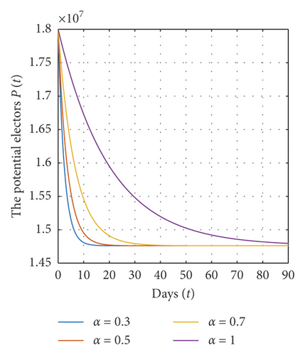
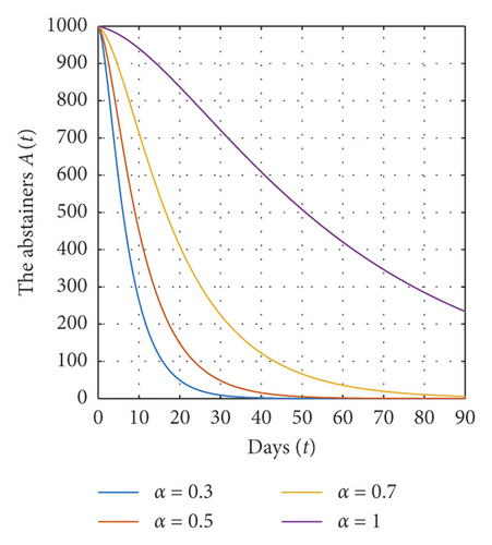
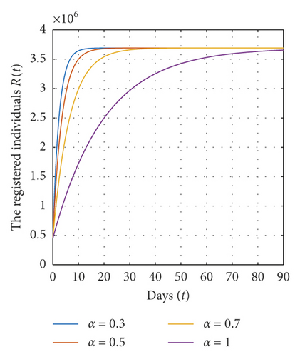
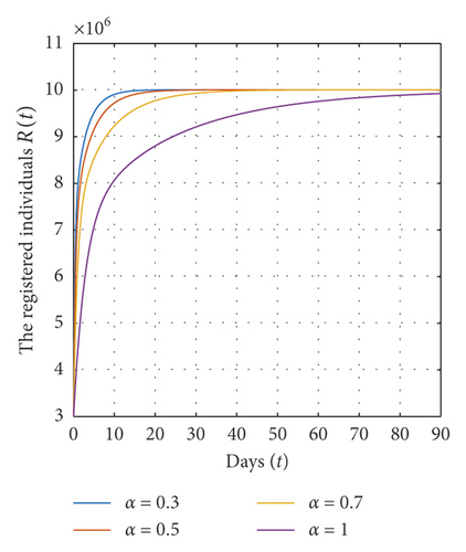
In this section, we present some numerical simulations of system (1) to illustrate our results. By choosing Λ = 73.8 × 10⁴, α = 0.01, β = 0.1, γ = 0.06, μ = 0.04, t_f = 90, and different values of α, we have the abstaining-free equilibrium E⁰ = (14.76 × 10⁶, 0,3.7 × 10⁶) and ℜ₀ = 0.8≺1. In this case, according to theorem (7), the abstaining-free equilibrium E⁰ of system (1) is globally asymptotically stable on Ω (see Figure 1).

Details are in the caption following the image — **Figure 1 (a)**
Open in figure viewer PowerPoint

Stability of the free equilibrium E⁰ for different values of α.

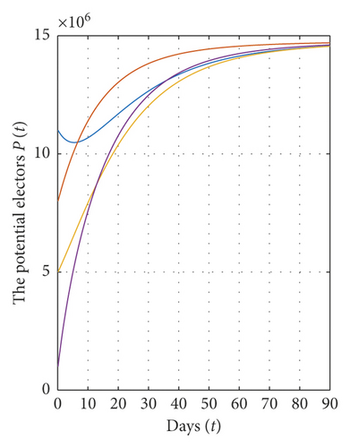
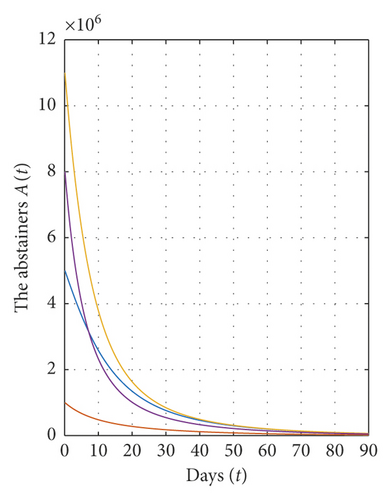
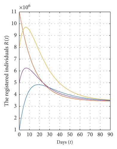
For a fixed value of α and for different initial values for each variable of state, we show in Figure 2 that the solutions converge to the abstaining-free equilibrium E⁰ = (14.76 × 10⁶, 0,3.7 × 10⁶) when ℜ₀ = 0.8≺1, which implies that the abstaining-free equilibrium E⁰ of system (1) is globally asymptotically stable on Ω.

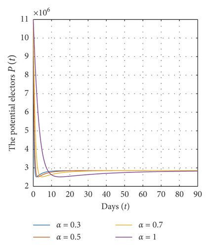
Concerning the stability analysis of the abstaining equilibrium E^∗, we have E^∗ = (2.85 × 10⁶, 6.1433 × 10⁶, 10.007 × 10⁶) and ℜ₀ = 1.79≻1 for Λ = 10.45 × 10⁵, α = 0.15, β = 0.5, γ = 0.02, μ = 0.055, and t_f = 90. In this case, according to theorem (9), the abstaining equilibrium E^∗ of system (1) is globally asymptotically stable on Ω (see Figure 3).

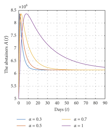
In addition, we show in Figure 4 that for a fixed value of α and for different initial values for each variable of state, the solutions converge to the abstaining equilibrium E^∗ = (2.85 × 10⁶, 6.1433 × 10⁶, 10.007 × 10⁶) and ℜ₀ = 1.79≻1, which implies that the abstaining equilibrium E^∗ of system (1) is globally asymptotically stable on Ω.

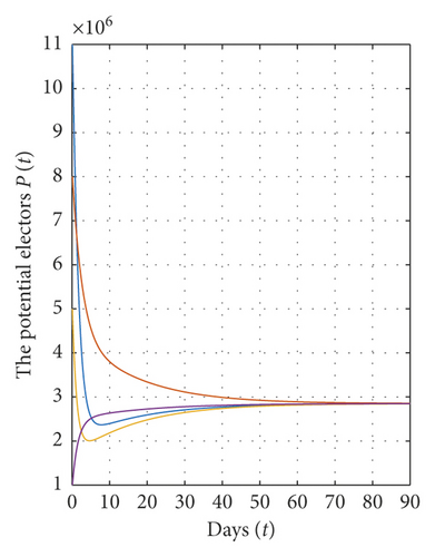
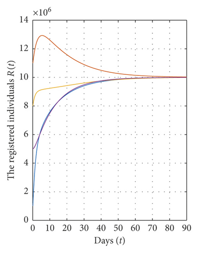
From all these figures, we show that the equilibrium points E⁰ and E^∗ of system (1) are globally asymptotically stable on Ω if the conditions of theorems (7) and (9) are satisfied. Also, all solutions of model (1) converge to the equilibrium points E⁰ and E^∗ for different values of α. In addition, the solutions converge rapidly to their steady state when the value of α is very small.

6. Conclusion

In this work, we presented a fractional-order model that describes the dynamics of citizens who have the right to register on the electoral lists and the negative influence of abstainers on the potential electors. By using the Routh–Hurwitz criteria and constructing Lyapunov functions, the local and the global stability of abstaining-free equilibrium and abstaining equilibrium are obtained. The numerical simulation was carried out using Matlab.

Conflicts of Interest

The authors declare that there are no conflicts of interest regarding the publication of this paper.

Open Research

Data Availability

The disciplinary data used to support the findings of this study have been deposited in the Network Repository (http://networkrepository.com/proÖle.php).

References

1 Leibniz G. W., Letter from hanover, Germany to G.F.A. L’Hospital, September 30, 1695, Leibniz Mathematische Schriften. (1962) Olms-Verlag, Hildesheim, Germany, 301–302.
Google Scholar
2 Leibniz G. W., Letter from hanover, Germany to john wallis, May 28, 1697, Leibniz Mathematische Schriften, 1962, Olms-Verlag, Hildesheim, Germany.
Google Scholar
3 Udita N. K., A new approach to generalized fractional derivatives, Bulletin of Mathematical Analysis and Applications. (2014) 6, no. 4, 1–15.
Google Scholar
4 Caputo M., Lectures on Seismology and Rheological Tectonics, 1992, Dipartimento di Fisica, Universita La Sapienza, Roma, Italy, Lecture Notes.
Google Scholar
5 El-Dessoky Ahmed M. M. and Altaf Khan M., Modeling and analysis of the polluted lakes system with various fractional approaches, Chaos, Solitons & Fractals. (2020) 134, 109720, https://doi.org/10.1016/j.chaos.2020.109720.
10.1016/j.chaos.2020.109720
Web of Science® Google Scholar
6 Khan M. A., Ahmad M., Ullah S., Farooq M., and Gul T., Modeling the transmission dynamics of tuberculosis in khyber pakhtunkhwa Pakistan, Advances in Mechanical Engineering. (2019) 11, no. 6, 168781401985483, https://doi.org/10.1177/1687814019854835, 2-s2.0-85067059426.
10.1177/1687814019854835
Web of Science® Google Scholar
7 Magin R., Fractional calculus in bioengineering, Cretical Reviews in Biomedical Engineering. (2004) 32, no. 3-4, https://doi.org/10.1615/critrevbiomedeng.v32.i34.10, 2-s2.0-11144305217.
10.1615/critrevbiomedeng.v32.i34.10
Google Scholar
8 Rossikhin Y. A. and Shitikova M. V., Applications of fractional calculus to dynamic problems of linear and nonlinear hereditary mechanics of solids, Applied Mechanics Reviews. (1997) 50, no. 1, 15–67, https://doi.org/10.1115/1.3101682, 2-s2.0-0030867045.
10.1115/1.3101682
Google Scholar
9 Scalas E., Gorenflo R., and Mainardi F., Fractional calculus and continuous-time finance, Physica A. Statistical Mechanics and Its Applications. (2000) 284, no. 1–4, 376–384, https://doi.org/10.1016/s0378-4371(00)00255-7, 2-s2.0-0034275979.
10.1016/S0378-4371(00)00255-7
Web of Science® Google Scholar
10 Song L., Xu S., and Yang J., Dynamical models of happiness with fractional order, Communications in Nonlinear Science and Numerical Simulation. (2010) 15, no. 3, 616–628, https://doi.org/10.1016/j.cnsns.2009.04.029, 2-s2.0-70349789880.
10.1016/j.cnsns.2009.04.029
Web of Science® Google Scholar
11 Ullah S., Khan M. A., Farooq M., and Gul T., Modeling and analysis of tuberculosis (TB) in khyber pakhtunkhwa, Pakistan, Mathematics and Computers in Simulation. (2019) 165, 181–199, https://doi.org/10.1016/j.matcom.2019.03.012, 2-s2.0-85064276995.
10.1016/j.matcom.2019.03.012
Web of Science® Google Scholar
12 Ullah S., Khan M. A., Altaf Khan M., Gul M. T., and Hussain F., A fractional order HBV model with hospitalization, Discrete & Continuous Dynamical Systems. (2020) 13, no. 3, 957–974, https://doi.org/10.3934/dcdss.2020056.
10.3934/dcdss.2020056
Web of Science® Google Scholar
13 Wang Z., Yang D., Ma T., and Sun N., Stability analysis for nonlinear fractional-order systems based on comparison principle, Nonlinear Dynamics. (2014) 75, no. 1-2, 387–402, https://doi.org/10.1007/s11071-013-1073-7, 2-s2.0-84891556704.
10.1007/s11071-013-1073-7
Web of Science® Google Scholar
14 Capponetto R., Dongola G., Fortuna L., and Petras I., Fractional order systems: modelling and control applications, World Scientific Series in Nonlinear Science, 2010, 72, Series A, Singapore, https://doi.org/10.1142/7709.
10.1142/7709
Google Scholar
15 Balatif O., Khajji B., and Rachik M., Mathematical modeling, analysis, and optimal control of abstinence behavior of registration on the electoral lists, Discrete Dynamics in Nature and Society. (2020) 2020, 12, 9738934, https://doi.org/10.1155/2020/9738934.
10.1155/2020/9738934
Web of Science® Google Scholar
16 Butzer P. L. and Westphal U., An introduction to fractional calculus, Applications of Fractional Calculus in Physics, 2000, World Scientific, River Edge, NJ, USA, 1–85, https://doi.org/10.1142/9789812817747_0001.
10.1142/9789812817747_0001
Web of Science® Google Scholar
17 Miller K. S. and Ross B., An Introduction to the Fractional Calculus and Fractional Differential Equations, 1993, John Wiley & Sons, New York, NY, USA.
Google Scholar
18 Oldham K. B. and Spanier J., The fractional calculus: theory and applications of differentiation and integration to arbitrary order, Mathematics in Science and Engineering. (1974) 11, Academic Press, London, UK.
Google Scholar
19 Podlubny I., Fractional differential equations, Mathematics in Science and Engineering. (1999) 198, Academic Press, San Diego, CA, USA.
Google Scholar
20 Odibat Z. M., Computing eigenelements of boundary value problems with fractional derivatives, Applied Mathematics and Computation. (2009) 215, no. 8, 3017–3028, https://doi.org/10.1016/j.amc.2009.09.049, 2-s2.0-70449531392.
10.1016/j.amc.2009.09.049
Web of Science® Google Scholar
21 Stojanovic M., Numerical method for solving diffusion-wave phenomena, Journal of Computational and Applied Mathematics. (2011) 235, 3121–3137, https://doi.org/10.1016/j.cam.2010.12.010, 2-s2.0-79952190735.
10.1016/j.cam.2010.12.010
Web of Science® Google Scholar
22 Lin W., Global existence theory and chaos control of fractional differential equations, Journal of Mathematical Analysis and Applications. (2007) 332, no. 1, 709–726, https://doi.org/10.1016/j.jmaa.2006.10.040, 2-s2.0-34247154280.
10.1016/j.jmaa.2006.10.040
Web of Science® Google Scholar
23 Bani-Yaghoub M., Gautam R., Shuai Z., van den Driessche P., and Ivanek R., Reproduction numbers for infections with free-living pathogens growing in the environment, Journal of Biological Dynamics. (2012) 6, no. 2, 923–940, https://doi.org/10.1080/17513758.2012.693206, 2-s2.0-84868316339.
10.1080/17513758.2012.693206
PubMed Web of Science® Google Scholar
24 Driessche P. V. and Watmough J., Reproduction numbers and sub-threshold endemic equilibria for compartmental models of disease transmission, Mathematical Biosciences. (2002) 180, no. 1-2, 29–48, https://doi.org/10.1016/s0025-5564(02)00108-6, 2-s2.0-0036845274.
10.1016/S0025-5564(02)00108-6
PubMed Web of Science® Google Scholar
25 Ahmed E., El-Sayed A. M. A., and El-Saka H. A. A., On some Routh-Hurwitz conditions for fractional order differential equations and their applications in Lorenz, Rössler, Chua and Chen systems, Physics Letters A. (2006) 358, no. 1, 1–4, https://doi.org/10.1016/j.physleta.2006.04.087, 2-s2.0-33746648126.
10.1016/j.physleta.2006.04.087
CAS Web of Science® Google Scholar
26 Boukhouima A., Hattaf K., and Yousfi N., A fractional order model for viral infection with cure of infected cells and humoral immunity, International Journal of Differential Equations. (2018) 2018, 1019242, https://doi.org/10.1155/2018/1019242, 2-s2.0-85058966994.
10.1155/2018/1019242
Google Scholar
27 Delavari H., Baleanu D., and Sadati J., Stability analysis of Caputo fractional-order nonlinear systems revisited, Nonlinear Dynamics. (2012) 67, no. 4, 2433–2439, https://doi.org/10.1007/s11071-011-0157-5, 2-s2.0-84858841611.
10.1007/s11071-011-0157-5
Web of Science® Google Scholar
28 De-Leon C. V., Volterra-type Lyapunov functions for fractional-order epidemic systems, Communications in Nonlinear Science and Numerical Simulation. (2015) 24, no. 1–3, 75–85, https://doi.org/10.1016/j.cnsns.2014.12.013, 2-s2.0-84924986295.
10.1016/j.cnsns.2014.12.013
Web of Science® Google Scholar
29 Tuan H. T. and Trinh H., Stability of fractional-order nonlinear systems by Lyapunov direct method, IET Control Theory & Applications. (2018) 12, no. 17, 2417–2422, https://doi.org/10.1049/iet-cta.2018.5233, 2-s2.0-85056355891.
10.1049/iet-cta.2018.5233
Web of Science® Google Scholar
30 Huo J., Zhao H., and Zhu L., The effect of vaccines on backward bifurcation in a fractional order HIV model, Nonlinear Analysis: Real World Applications. (2015) 26, 289–305, https://doi.org/10.1016/j.nonrwa.2015.05.014, 2-s2.0-84933529409.
10.1016/j.nonrwa.2015.05.014
Web of Science® Google Scholar
31 LaSalle J. P., The stability of dynamical systems, Regional Conference Series in Applied Mathmatics. (1976) 25, SIAM, Newdelhi, India.
Google Scholar

Citing Literature

All articles

Stability Analysis of a Fractional-Order Model for Abstinence Behavior of Registration on the Electoral Lists

Abstract

1. Introduction

2. Preliminaries

3. Basic Properties of the Model

4. Stability Analysis

4.1. Local Stability Analysis

4.2. Global Stability Analysis

5. Numerical Simulation

6. Conclusion

Conflicts of Interest

Open Research

Data Availability

References

Citing Literature

Figures

References

Information

About Wiley Online Library

Help & Support

Opportunities

Connect with Wiley

Stability Analysis of a Fractional-Order Model for Abstinence Behavior of Registration on the Electoral Lists

Abstract

1. Introduction

2. Preliminaries

3. Basic Properties of the Model

4. Stability Analysis

4.1. Local Stability Analysis

4.2. Global Stability Analysis

5. Numerical Simulation

6. Conclusion

Conflicts of Interest

Open Research

Data Availability

References

Citing Literature

Figures

References

Related

Information