Volume 2019, Issue 1 9303676

Research Article

Open Access

Bearing Fault Diagnosis Using a Support Vector Machine Optimized by an Improved Ant Lion Optimizer

Corresponding Author

Dalian Yang

[email protected]

orcid.org/0000-0003-0444-3653

Hunan Provincial Key Laboratory of Health Maintenance for Mechanical Equipment, Hunan University of Science and Technology, Xiangtan 411201, China hnust.edu.cn

Engineering Research Center of Advanced Mining Equipment, Ministry of Education, Hunan University of Science and Technology, Xiangtan 411201, China hnust.edu.cn

Search for more papers by this author

Jingjing Miao,

Jingjing Miao

orcid.org/0000-0002-8586-5462

Hunan Provincial Key Laboratory of Health Maintenance for Mechanical Equipment, Hunan University of Science and Technology, Xiangtan 411201, China hnust.edu.cn

Search for more papers by this author

Fanyu Zhang,

Fanyu Zhang

orcid.org/0000-0002-8709-2539

Hunan Provincial Key Laboratory of Health Maintenance for Mechanical Equipment, Hunan University of Science and Technology, Xiangtan 411201, China hnust.edu.cn

Search for more papers by this author

Jie Tao,

Jie Tao

orcid.org/0000-0002-1444-8709

Key Laboratory of Knowledge Processing and Networked Manufacturing, Hunan University of Science and Technology, Xiangtan 411201, China hnust.edu.cn

Search for more papers by this author

Guangbin Wang,

Guangbin Wang

orcid.org/0000-0002-1531-3275

Hunan Provincial Key Laboratory of Health Maintenance for Mechanical Equipment, Hunan University of Science and Technology, Xiangtan 411201, China hnust.edu.cn

Engineering Research Center of Advanced Mining Equipment, Ministry of Education, Hunan University of Science and Technology, Xiangtan 411201, China hnust.edu.cn

Search for more papers by this author

Yiping Shen,

Yiping Shen

orcid.org/0000-0001-9073-7900

Hunan Provincial Key Laboratory of Health Maintenance for Mechanical Equipment, Hunan University of Science and Technology, Xiangtan 411201, China hnust.edu.cn

Engineering Research Center of Advanced Mining Equipment, Ministry of Education, Hunan University of Science and Technology, Xiangtan 411201, China hnust.edu.cn

Search for more papers by this author

Dalian Yang,

Corresponding Author

Dalian Yang

[email protected]

orcid.org/0000-0003-0444-3653

Hunan Provincial Key Laboratory of Health Maintenance for Mechanical Equipment, Hunan University of Science and Technology, Xiangtan 411201, China hnust.edu.cn

Engineering Research Center of Advanced Mining Equipment, Ministry of Education, Hunan University of Science and Technology, Xiangtan 411201, China hnust.edu.cn

Search for more papers by this author

Jingjing Miao,

Jingjing Miao

orcid.org/0000-0002-8586-5462

Hunan Provincial Key Laboratory of Health Maintenance for Mechanical Equipment, Hunan University of Science and Technology, Xiangtan 411201, China hnust.edu.cn

Search for more papers by this author

Fanyu Zhang,

Fanyu Zhang

orcid.org/0000-0002-8709-2539

Hunan Provincial Key Laboratory of Health Maintenance for Mechanical Equipment, Hunan University of Science and Technology, Xiangtan 411201, China hnust.edu.cn

Search for more papers by this author

Jie Tao,

Jie Tao

orcid.org/0000-0002-1444-8709

Key Laboratory of Knowledge Processing and Networked Manufacturing, Hunan University of Science and Technology, Xiangtan 411201, China hnust.edu.cn

Search for more papers by this author

Guangbin Wang,

Guangbin Wang

orcid.org/0000-0002-1531-3275

Hunan Provincial Key Laboratory of Health Maintenance for Mechanical Equipment, Hunan University of Science and Technology, Xiangtan 411201, China hnust.edu.cn

Engineering Research Center of Advanced Mining Equipment, Ministry of Education, Hunan University of Science and Technology, Xiangtan 411201, China hnust.edu.cn

Search for more papers by this author

Yiping Shen,

Yiping Shen

orcid.org/0000-0001-9073-7900

Hunan Provincial Key Laboratory of Health Maintenance for Mechanical Equipment, Hunan University of Science and Technology, Xiangtan 411201, China hnust.edu.cn

Engineering Research Center of Advanced Mining Equipment, Ministry of Education, Hunan University of Science and Technology, Xiangtan 411201, China hnust.edu.cn

Search for more papers by this author

First published: 2019

https://doi.org/10.1155/2019/9303676

Citations: 7

Academic Editor: Zhixiong Li

Share a link

Email
Wechat
Bluesky

Abstract

Bearing is an important mechanical component that easily fails in a bad working environment. Support vector machines can be used to diagnose bearing faults; however, the recognition ability of the model is greatly affected by the kernel function and its parameters. Unfortunately, optimal parameters are difficult to select. To address these limitations, an escape mechanism and adaptive convergence conditions were introduced to the ALO algorithm. As a result, the EALO method was proposed and has been applied to the more accurate selection of SVM model parameters. To assess the model, the vibration acceleration signals of normal, inner ring fault, outer ring fault, and ball fault bearings were collected at different rotation speeds (1500 r/min, 1800 r/min, 2100 r/min, and 2400 r/min). The vibration signals were decomposed using the variational mode decomposition (VMD) method. The features were extracted through the kernel function to fuse the energy value of each VMD component. In these experiments, the two most important parameters for the support vector machine—the Gaussian kernel parameter σ and the penalty factor C—were optimized using the EALO algorithm, ALO algorithm, genetic algorithm (GA), and particle swarm optimization (PSO) algorithm. The performance of these four methods to optimize the two parameters was then compared and analyzed, with the EALO method having the best performance. The recognition rates for bearing faults under different tested rotation speeds were improved when the SVM model parameters optimized by the EALO were used.

1. Introduction

The rolling bearing is a core mechanical component that is widely used in wind turbines, aeroengines, ships, automobiles, and other important mechanical equipment [1, 2]. Rolling bearings usually perform for extended periods of time in extreme conditions such as high temperatures, high speeds, and high loading. These long-term, extreme running conditions lead to a variety of serious failures, including ball bearing wear, metal spalling on the inner and outer raceways, and cracks in the cage [3]. A weak fault results in abnormal vibrations, which hinder the performance of the mechanical equipment and reduce work efficiency. A serious fault may result in the destruction of the machine and—depending on the severity—lead to employee death. Whether a mechanical malfunction or human injury and/or death, the result is a huge loss to the business enterprise and society as a whole; ultimately, this results in a serious barrier to the harmonious development of a national economy. Although bearing failure is inevitable, abiding by a standard maintenance schedule can partially reduce the accident rate caused by bearing failure. However, bearings still suffer issues of over- and undermaintenance, resulting in increased business costs. Developments in computer and testing technology have led to many advanced automatic monitoring and intelligent diagnostics. These have been adopted to allow for online monitoring of working conditions, which allow for timely fault detection as well as the development of accurate reference points for future maintenance decisions. Given these advantages, it is important to study the application of intelligent fault diagnostic technology to rolling bearing performance.

Currently, the vibration monitoring method is the most commonly adopted method to monitor bearing conditions [4]. When the fault first appears, its characteristic signal is very weak [5]. This is because it is overwhelmed by the power of the natural frequency vibrations, transfer modulation, and noise interference. Despite being weak, the signal has obvious nonlinear and nonstationary characteristics [6]. Traditional fault diagnostic methods include analyzing vibration signals from the time, frequency, and time-frequency domains. Traditional approaches have difficulty detecting these signals because they are based on the neural network [7–9] and the Bayesian decision [10–12] methods, which require a large number of valid samples to function properly. This means that when the sample size is too small, model accuracy decreases; however, a large number of fault samples are difficult to discern. Therefore, the application of traditional pattern recognition methods such as the neural network and the Bayesian decision is restricted.

The support vector machine (SVM) [13–15] is a pattern recognition method developed in the 1990s that is suitable for small sample conditions. This method takes a kernel function as the core and implicitly maps the original data of the original space to the feature space. In this manner, a search for linear relations in the feature space is conducted, which can then determine efficient solutions to nonlinear problems. SVM has been widely applied in the field of pattern recognition and has been applied to such problems as text recognition [16], handwritten numeral recognition [17], face detection [18], system control [19], and many other related applications. The accuracy of SVM classification is highly affected by the kernel function and its parameters since the relationship between the parameters and model classification accuracy in a multimodal function is irregular. Given this, improper parameter values worsen the model’s generalization ability, leading to more inaccurate fault recognition. Unfortunately, it is difficult to obtain optimal parameters. When applied, empirical selection is unreliable. Computer-driven parameter optimization not only reduces the workload of human engineers but also provides a more reliable basis for the selection of optimal solutions. Current methods used for parameter optimization include grid cross-validation (GCV) [20, 21], genetic algorithm (GA) [22], and particle swarm optimization (PSO) [23, 24]; despite this variety, the optimization efficiency of these methods remains imperfect.

In 2015, a new bionic intelligent algorithm termed “Ant Lion Optimizer” (ALO) was devised by Mirjalili [25]. ALO has many advantages, including its simple principle, ease of implementation, reduced need for parameter adjustment, and high precision [26, 27]. It has been successfully applied to a variety of fields like structure optimization [28], antenna layout optimization [29], distributed system siting [30], idle power distribution problem [31], community mining in complex networks [32], and feature extraction [33]. Recently, He et al. [34] utilized the ant lion optimizer to optimize a GM (1,1) model to predict the power demands of Beijing. Their results showed that this approach improved the adaptability of the GM (1,1) model. Relatedly, Zhao et al. [35] improved the ant lion optimizer by using a chaos detection mechanism to optimize SVM. They then used a UCI standard database for verification. Collectively, their results showed the ALO algorithm improved classification accuracy.

At present, there are few studies regarding ALO application in bearing fault diagnosis. As a new bionic optimization algorithm, there are some ant lion individuals in the ALO algorithm with relatively poor fitness in the iteration process. If the ants select poor fitness ant lions for walking, the probability of falling into a local extremum increases. In addition, resource waste will result if poor fitness ant lions search around the local extremum and partially affect the optimization performance and convergence efficiency of the ALO algorithm.

Given the aforementioned problems, this paper uses the rolling bearing as its test object and to improve the ant lion algorithm. When combined with SVM, it also sought to diagnose bearing faults. This work has both great theoretical significance and practical value to improve the accuracy of fault diagnosis in rolling bearings, thereby ensuring the safety and stability of functional rolling bearings.

2. Basic Algorithm Principles

2.1. Ant Lion Optimizer

The ALO algorithm was modeled on the hunting behavior of ant larvae in nature. As constructed, the optimization algorithm mimics the walking of random ants, constructs traps, lures the ants into the trap, captures the ants, and reconstructs the traps. The ALO algorithm conducts a global search by walking around randomly selected ant lions, and local refinement optimization is achieved by adaptive boundary of the ant lion trap.

The total number of ants and ant lions is defined by N, the problem dimension is D, the maximum number of iterations is I_ter, the lower boundary of the optimal space is

L^{k} = [l_{1}^{k}, l_{2}^{k}, l_{3}^{k}, \dots, l_{D}^{k}]

, the upper boundary is

U^{k} = [u_{1}^{k}, u_{2}^{k}, u_{3}^{k}, \dots, u_{D}^{k}]

, the position matrix of ants is

M_{ant}^{k}

, and the position matrix of ant lions is

M_{antlion}^{k}

\begin{matrix} M_{ant}^{k} = [\begin{matrix} M_{{ant}_{1}}^{k} \\ M_{{ant}_{2}}^{k} \\ ⋮ \\ M_{{ant}_{N}}^{k} \end{matrix}] = [\begin{matrix} A_{{ant}_{11}}^{k} & A_{{ant}_{12}}^{k} & \dots & A_{{ant}_{1 D}}^{k} \\ A_{{ant}_{21}}^{k} & A_{{ant}_{22}}^{k} & \dots & A_{{ant}_{2 D}}^{k} \\ ⋮ & ⋮ & ⋮ & ⋮ \\ A_{{ant}_{N 1}}^{k} & A_{{ant}_{N 2}}^{k} & \dots & A_{{ant}_{N D}}^{k} \end{matrix}], \\ M_{antlion}^{k} = [\begin{matrix} M_{{antlion}_{1}}^{k} \\ M_{{antlion}_{2}}^{k} \\ ⋮ \\ M_{{antlion}_{N}}^{k} \end{matrix}] = [\begin{matrix} A_{{antlion}_{11}}^{k} & A_{{antlion}_{12}}^{k} & \dots & A_{{antlion}_{1 D}}^{k} \\ A_{{antlion}_{21}}^{k} & A_{{antlion}_{22}}^{k} & \dots & A_{{antlion}_{2 D}}^{k} \\ ⋮ & ⋮ & ⋮ & ⋮ \\ A_{{antlion}_{N 1}}^{k} & A_{{antlion}_{N 2}}^{k} & \dots & A_{{antlion}_{N D}}^{k} \end{matrix}], \end{matrix}

()

where k represents the current number of iterations and satisfies 0 ≤ k ≤ I_ter,

A_{{ant}_{i j}}^{k}

represents the position of the i-th ant in the j-th dimensional space after the k-th iteration, and

A_{{antlion}_{i j}}^{k}

represents the position of the i-th ant lion in the j-th dimension space after the k-th iteration. When k = 0, the position of the initial ant and ant lion populations can be assigned by the following formulae:

\begin{matrix} A_{{ant}_{i j}}^{0} = rand () \times (u_{j}^{0} - l_{j}^{0}) + l_{j}^{0}, \end{matrix}

()

\begin{matrix} A_{{antlion}_{i j}}^{0} = rand () \times (u_{j}^{0} - l_{j}^{0}) + l_{j}^{0} . \end{matrix}

()

The fitness vectors

F_{ant}^{k}

and

F_{antlion}^{k}

can be expressed as

\begin{matrix} F_{ant}^{k} = [\begin{matrix} F_{ant_{fitness}_{1}}^{k} \\ F_{ant_{fitness}_{2}}^{k} \\ ⋮ \\ F_{ant_{fitness}_{N}}^{k} \end{matrix}] = [\begin{matrix} f ([A_{{ant}_{11}}^{k}, A_{{ant}_{12}}^{k}, \dots, A_{{ant}_{1 D}}^{k}]) \\ f ([A_{{ant}_{21}}^{k}, A_{{ant}_{22}}^{k}, \dots, A_{{ant}_{2 D}}^{k}]) \\ ⋮ \\ f ([A_{{ant}_{N 1}}^{k}, A_{{ant}_{N 2}}^{k}, \dots, A_{{ant}_{N D}}^{k}]) \end{matrix}], \\ F_{antlion}^{k} = [\begin{matrix} F_{antlion_{fitness}_{1}}^{k} \\ F_{antlion_{fitness}_{2}}^{k} \\ ⋮ \\ F_{antlion_{fitness}_{N}}^{k} \end{matrix}] = [\begin{matrix} f ([A_{{antlion}_{11}}^{k}, A_{{antlion}_{12}}^{k}, \dots, A_{{antlion}_{1 D}}^{k}]) \\ f ([A_{{antlion}_{21}}^{k}, A_{{antlion}_{22}}^{k}, \dots, A_{{antlion}_{2 D}}^{k}]) \\ ⋮ \\ f ([A_{{antlion}_{N 1}}^{k}, A_{{antlion}_{N 2}}^{k}, \dots, A_{{antlion}_{N D}}^{k}]) \end{matrix}], \end{matrix}

()

where f(⋅) is the fitness evaluation function. Define

E_{elite}^{k}

as the elite ant lion after the k-th iteration, which satisfies

\begin{matrix} f (E_{elite}^{k}) = \max (F_{antlion}^{k}) . \end{matrix}

()

The iterative process of the ALO algorithm is to continuously update the position according to the interaction between the ants and the ant lions; after this update, it then reselects the elite ant lions. The ALO algorithm primarily includes random ant walks, trapping in an ant lion’s pit, building traps, sliding ants towards the ant lion, catching prey, rebuilding the pit, and elitism.

2.1.1. Random Ant Walks

When searching for food in nature, ants move stochastically; as such, a random walk X(t) is used to model ants’ movement as follows:

\begin{matrix} X^{k} = [0, \sum_{k = 0}^{0} (21 r (k) -), \sum_{k = 0}^{1} (21 r (k) -), \dots, \sum_{k = 0}^{I_{ter}} (21 r (k) -)], \end{matrix}

()

where r(⋅) is a stochastic function that is defined as follows:

\begin{matrix} r (\cdot) = \{\begin{cases} 1, & if rand () \geq 0.5, \\ 0, & if rand () < 0.5. \end{cases} \end{matrix}

()

In order to ensure the random walks of ants in the search space, the position of the ants is normalized by

\begin{matrix} X_{norm}^{k} = \frac{(X^{k} - \min (X^{k})) \times (u_{j}^{k} - l_{j}^{k})}{(\max (X^{k}) - \min (X^{k}))} + l_{j}^{k} . \end{matrix}

()

2.1.2. Building a Trap

According to its fitness, an individual ant lion is selected from the ant lion population of the previous generation through a roulette operation, defined as follows:

\begin{matrix} W^{k} = \frac{1}{sort (F_{antlion}^{k})}, \end{matrix}

()

where sort(⋅) is the sorting function (in positive order), which is defined as

\begin{matrix} P = [\sum_{i = 1}^{1} W_{i}^{k}, \sum_{i = 1}^{2} W_{i}^{k}, \dots, \sum_{i = 1}^{N} W_{i}^{k}], \end{matrix}

()

\begin{matrix} {Ind}_{i} = P_{i} - P_{N} \times rand () . \end{matrix}

()

As i increases from 1 and when the first Ind_i > 0 is satisfied, $A_{{antlion}_{i}}^{k}$ is the selected individual, which then builds the trap together with the elite named “ $E_{roulette}^{k}$ .”

2.1.3. Trapping in an Ant Lion’s Pit

This process is described as the ants walking around the “trap.” The boundary of the walking area is affected by the position of the elite, which can be defined by the following formula:

\begin{matrix} \{\begin{cases} L^{k} = E_{elite}^{k} + L^{k}, \\ U^{k} = E_{elite}^{k} + U^{k} . \end{cases} \end{matrix}

()

2.1.4. Sliding Ants towards the Ant Lion

As soon as the ant starts sliding towards the trap, the ant lions realize the ant is in the trap and shoot sand to the center of the pit to prevent it from escaping. The process can be described as an adaptive decrease in the radius of a given ant’s random walk hypersphere:

\begin{matrix} \{\begin{cases} L^{k} = \frac{L^{k} I_{ter}}{G 10^{w}}, \\ U^{k} = \frac{U^{k} I_{ter}}{G 10^{w}}, \end{cases} \end{matrix}

()

where G is the ratio of the current iteration number to the maximum iteration number and w is the radius reduction scale index, which satisfies

\begin{matrix} w = \{\begin{cases} 1, & G < 0.1 I_{ter}, \\ 2, & 0.10.5 I_{ter} \leq G < I_{ter}, \\ 3, & 0.50.75 I_{ter} \leq G < I_{ter}, \\ 4, & 0.750.9 I_{ter} \leq G < I_{ter}, \\ 5, & 0.90.95 I_{ter} \leq G < I_{ter}, \\ 6, & 0.95 I_{ter} \leq G . \end{cases} \end{matrix}

()

2.1.5. Catching Prey and Rebuilding the Pit

The ant lion kills the ant and eats its body. If a prey ant’s fitness is higher than the elite’s fitness, the elite ant lions update their position to the prey ants. In other words, the elite ant lions will build new traps for the next prey. Given this scenario, the following equation is proposed:

\begin{matrix} E_{elite}^{k} = M_{{ant}_{i}}^{k}, if f (E_{elite}^{k}) > f (M_{{ant}_{i}}^{k}) . \end{matrix}

()

2.1.6. Elitism

The elite ant lion affects the movements of all ants, with each ant randomly walking around a selected ant lion; this walking is done according to both the roulette wheel and the elite, simultaneously. This behavior is modeled according to the following function:

\begin{matrix} M_{{ant}_{i}}^{k} = \frac{R_{roulette}^{k} + R_{elite}^{k}}{2}, \end{matrix}

()

where

R_{roulette}^{k}

represents the ant lions which are selected by the roulette wheel at the k-th iteration and

R_{elite}^{k}

represents the ants who walk around the elite at the k-th iteration.

2.2. Support Vector Machine

In the 1950s, Vapnik [13] proposed a new machine learning method that was termed the support vector machine (SVM). SVM is based on both the statistical learning theory and the structural risk minimization principle. Statistical learning theory is specialized for small sample situations of machine learning theory; given this, SVM has a good generalization ability. In addition, SVM is a convex quadratic optimization problem, which guarantees that the obtained extremum solution is also the global optimal solution [36, 37]. Collectively, these characteristics allow it to avoid the local extremum and dimensional disaster problems that are unavoidable when using a neural network. The standard SVM model has been established for two types of classification samples. Its basic principles are as follows.

For the two types of classes to be classified, the sample dataset is defined as follows:

\begin{matrix} X = \{(x_{i}, y_{i})\}, i = 1,2,3, \dots, n, x_{i} \in R^{n}, y_{i} \in \{+ 1,1\} . \end{matrix}

()

The establishment of an SVM classification model is done to find an optimal classification surface ω, which satisfies

\begin{matrix} ω \cdot x + b = 0, \end{matrix}

()

where ω is the normal vector of the hyperplane and b is the offset vector. Therefore, the following convex quadratic optimization model can be established:

\begin{matrix} \{\begin{cases} \min \frac{{‖ω‖}^{2}}{2} + C \sum_{i = 1}^{n} ξ_{i} \\ st . y_{i} [(ω \cdot x_{i}) + b] - 10 \geq, \end{cases} \end{matrix}

()

where C is the punishment factor and ξ_i is the relaxation factor.

By solving the following dual problem, the optimal solution α^∗ is obtained:

\begin{matrix} \{\begin{cases} \max \sum_{i = 0}^{n} α_{i} - \frac{\sum_{i = 1}^{n} \sum_{j = 1}^{n} α_{i} α_{j} y_{i} y_{j} 〈x_{i}, x_{j}〉}{2} \\ s . t . \sum_{i = 1}^{n} α_{i} y_{i} = 0 \\ 01,2,3 \leq α_{i} \leq C, i =, \dots, n . \end{cases} \end{matrix}

()

This allows the optimal hyperplane normal vector in equation (19) to be obtained:

\begin{matrix} ω^{*} = \sum_{i = 1}^{n} α_{i}^{*} y_{i} x_{i} . \end{matrix}

()

The corresponding samples to

0 < α_{i}^{*} < C

are called the support vectors (SVs), and the offset vector is calculated by

\begin{matrix} b^{*} = y_{i} - \sum_{i = 1}^{l} y_{i} α_{i} 〈x_{i}, x_{j}〉 . \end{matrix}

()

The decision function yielded is as follows:

\begin{matrix} f (x) = sgn (\sum_{i = 1}^{n} α_{i}^{*} y_{i} 〈x, x_{i}〉 + b^{*}) . \end{matrix}

()

The above SVM model has been established for linear sample classification; for nonlinear classification, the nonlinear transform Φ : Rⁿ⟶H, x⟶Φ(x) is introduced. Φ can transform the nonlinear samples in low-dimensional space into linear samples in high-dimensional Hilbert space. Unfortunately, this nonlinear transformation is difficult to obtain. In practice, a kernel function K(x_i, x_j) is often used instead of the explicit nonlinear transform equation Φ. The kernel function transforms the nonlinear samples in low-dimensional space into high-dimensional Hilbert space by calculating the inner product. So the discriminant function is described as

\begin{matrix} f (x) = sgn (\sum_{i = 1}^{n} α_{i}^{*} y_{i} K (x_{i}, x_{j}) + b^{*}) . \end{matrix}

()

As shown in formula (24), the kernel function is the core of the SVM, and it plays an important role in its generalization ability. The common kernel functions are shown in Table 1.

Table 1. Common kernel function expressions and parameters.

Kernel functions	Expressions	Parameters
Linear kernel	$K (x_{i}, x_{j}) = x_{i}^{T} x_{j}$	None
Polynomial kernel	$K (x_{i}, x_{j}) = {(x_{i}^{T} x_{j} + l)}^{d}$	l ∈ R; d ∈ Z⁺
Gauss kernel	$K (x_{i}, x_{j}) = \exp (- {‖x_{i} - x_{j}‖}^{2} / 2 σ^{2})$	σ > 0
Sigmoid kernel	$K (x_{i}, x_{j}) = \tan (β x_{i}^{T} x_{j} + b)$	β ≠ 0; b ∈ R

As shown in Table 1, different kernel functions have different expressions and parameters. Therefore, different kernel functions and parameters have different abilities to map data to higher-dimensional space. Since kernel functions and parameter values affect the generalization ability of the SVM model, the selection of the best parameters is extremely important.

The standard SVM solves the problem of two-class classification; in reality, encountering a multiclass problem is more common than a two-class problem. Therefore, the study of a multiclass SVM problem is of great significance. At present, researchers have proposed a handful of effective multiclass SVM construction methods. These approaches can be divided into two categories, with the first being the direct construction method. This method improves the discriminant function of a two-class SVM model to construct a multiclass model. This method uses only one SVM discriminant function to achieve a multiclass output. The discriminant function of this algorithm is very complex, and its classification accuracy is not good. The second method is to realize the construction of a multiclass SVM classifier by combining multiple two-class SVMs. In practice, this method is more widely used and includes one-against-one, one-against-all, direct acyclic graph, and binary tree approaches [38].

3. Ant Lion Optimizer Improvement

3.1. Improvement Based on the Escape Mechanism

In the ALO algorithm, ants randomly walk around the elite ant lion and the roulette wheel-selected ant lion; these ants gradually fall into the trap set by the ant lion. As the number of iterations increases, the walk range of the ants becomes increasingly smaller. In turn, this means the range of the search optimization solution becomes increasingly smaller as well. If the elite ant lion is located at the local extremum value, the risk of falling into the local extremum is increased. This reduces the optimization performance of the ALO algorithm. In nature, when an ant lion builds an ant trap, it is not always successful in catching the ants that fall into the trap. If the ants find that there is an ant lion nearby, they will avoid it to escape being eaten.

Here—and based on the aforementioned considerations—the ant escape mechanism was introduced into the ALO algorithm. This introduction resulted in an improved ALO algorithm, termed here as the EALO algorithm. By introducing the ant escape mechanism, the possibility of the algorithm falling into a local extremum value is reduced, thereby improving the optimization ability of the algorithm.

P_esc is defined as the escape probability of the ants, N is the maximum number of ants, and N_esc is the maximum number of escaped ants, satisfying N_esc ≤ N. The fitness of the ants

F_{ant}^{k}

is ranked after walking around the elite ant lion and the roulette-selected ant lion, where k is the iteration number. Then, the former N_esc ants with low fitness are selected and randomly assigned to any location within the search field. That is,

\begin{matrix} A_{esc_{ant}_{i j}}^{k} = rand () \times (u_{b j}^{0} - l_{b j}^{0}) + l_{b j}^{0}, if rand () > P_{esc}, \end{matrix}

()

where i = 1,2, …, N_esc and j = 1,2, …, D.

3.2. Improvement Based on Adaptive Convergence Conditions

The optimization performance of the ALO algorithm includes primarily precision and time consumption. In the ALO algorithm, algorithm convergence is controlled by setting the maximum number of iterations I_ter. If the maximum preset number of iterations is too large, the algorithm will take too long to complete; if the maximum number of iterations is too small, the precision of the algorithm cannot be guaranteed. For this reason, I_ter usually takes a large value in practical applications, with algorithm accuracy taking priority over time. However, some applications like online monitoring and fault diagnosis require more accurate solutions that are obtained in a short time. This is because it is necessary to have rapid assessment of the running state of mechanical equipment. Given this, it is unreasonable to adopt a fixed number of iterations. This is because as the number of iterations increases, the walking range of the ants will decrease; moreover, fitness differences between individuals will also decrease.

Assuming that ε is a small positive number, if the following formula is satisfied, then the EALO algorithm terminates and returns an optimal solution

E_{elite}^{k}

\begin{matrix} threshold = |\max (F_{ant}^{k}) - \min (F_{ant}^{k})| < ε, k \geq 2. \end{matrix}

()

4. EALO-SVM Modeling

Assuming that S = {S₁, S₂, S₃, …, S_n} is a sample set containing n-class faults, the same number of samples are randomly selected from each fault sample set to form the training sample set S¹. The rest of the samples form the test sample set S². Taking the radial basis kernel function as an example, the parameters that need to be optimized are the kernel function parameter σ and penalty factor C. A diagram of the SVM parameter optimization based on EALO is shown in Figure 1, and the modeling steps are as follows:

(1)
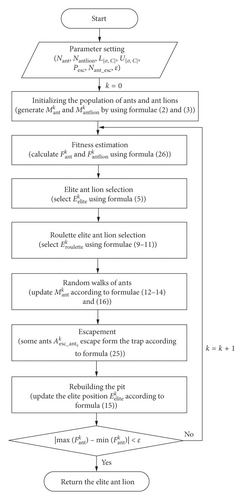
Parameter Presetting. Set the population number of ants as N_ant and the population number of ant lions as N_antlion. The lower boundary of the searching space is $L_{\{σ, C\}}^{0} = [l_{σ}^{0}, l_{C}^{0}]$ . The upper boundary of the searching space is $U_{\{σ, C\}}^{0} = [u_{σ}^{0}, u_{C}^{0}]$ . The probability of ant escape is P_esc, the maximum number of ants to escape is N_{ant_esc}, and the convergence threshold is ε.
(2)
Ant and Ant Lion Population Initialization. According to the preset parameters and the parameters {σ, C} to be optimized, the ant position matrix $M_{ant}^{k}$ and ant lion position matrix $M_{antlion}^{k}$ are randomly generated according to formula (2) and formula (3).
(3)
Fitness Estimation. According to the ant position matrix $M_{ant}^{k}$ and the ant lion position matrix $M_{antlion}^{k}$ , training the SVM model uses the sample set S¹ and then predicts the testing sample set S². The fitness vectors $F_{ant}^{k}$ of the ant and $F_{antlion}^{k}$ of the ant lion are obtained. Thereby, the fitness estimation function f(⋅) is defined by the following formula:
$\begin{matrix} \{\begin{cases} F_{ant}^{k} = f (\cdot) = SVM_Predict (SVM_Train (M_{ant}^{k}, S^{1}), S^{2}), \\ F_{antlion}^{k} = f (\cdot) = SVM_Predict (SVM_Train (M_{antlion}^{k}, S^{1}), S^{2}) . \end{cases} \end{matrix}$ ()
(4)
Natural Elite Selection. According to formula (5), the ant lion with the highest fitness is selected as the natural elite ant lion $E_{elite}^{k}$ .
(5)
Roulette Elite Selection. According to formulae (9)–(11), roulette elite ant lions $E_{roulette}^{k}$ were selected.
(6)
Ant Random Walking. According to formulae (12)–(14), ants randomly walking around the natural elite ant lions are $E_{elite}^{k}$ and roulette elite ant lions are $E_{roulette}^{k}$ .
(7)
Random Escape. Some ants are randomly assigned to any position in the searching space according to formula (25).
(8)
Rebuilding the Traps. After feeding on the ants, the position of the natural elite ant lion is updated according to formula (15). The natural elite ant lion continues to rebuild traps in the new position to prepare for the next predation.
(9)
Stopping the Iteration. To calculate the maximum and minimum fitness of the ants, formula (26) is used. If formula (26) is not true, then return to step (5) and continue to the next iteration. Otherwise, the iteration is stopped and output the natural elite ant lions $E_{elite}^{k^{*}}$ ; its position is taken as the optimal solution {σ^∗, C^∗}.

Details are in the caption following the image — **Figure 1**
Open in figure viewer PowerPoint

Flow diagram of the EALO-SVM algorithm.

5. Experiments

5.1. Data Acquisition

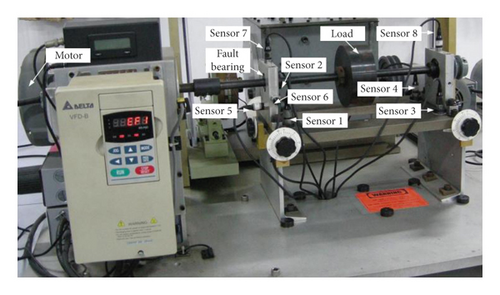
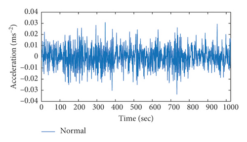
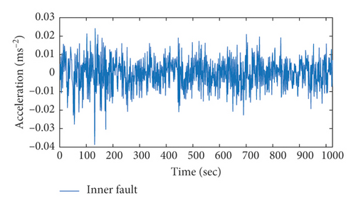
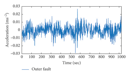
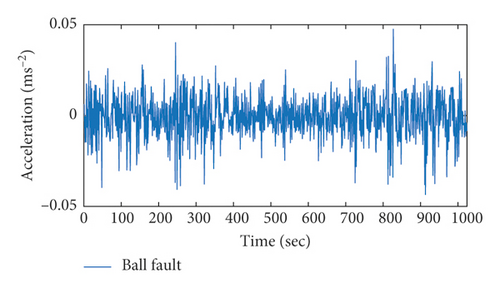
Bearing fault vibration tests were conducted to verify the performance of the EALO-SVM algorithm. These tests were performed on a machinery fault simulator (SpectraQuest Inc., Hermitage Road, Richmond, Virginia, USA) and are shown in Figure 2. The simulator is driven by a three-phase motor and allows for accurate control of the rotation speed. In the experiment, the fault bearing was installed on the bearing pedestal near the motor, and the normal bearing was installed on the right bearing pedestal. The vibration signals were collected using a high-speed multichannel data acquisition instrument (DEWETRON, Graz, Austria). Eight acceleration sensors were installed: Four of them were installed on the base (sensors 1–4), three on the fault-bearing pedestal to obtain vibration acceleration signals in the x, y, and z directions (sensors 5–7), and one on the other bearing pedestal (sensor 8). The sampling frequency was 10 kHz. Four typical bearing faults (normal, inner ring, outer ring, and ball) were simulated at four motor speeds (1500, 1800, 2100, and 2400 r/min), and their vibration acceleration signals were collected. The time waveform of the partially collected acceleration signal is shown in Figure 3.

5.2. Feature Extraction

As shown in Figure 3, bearing fault signals were highly nonlinear and nonstationary, making it difficult to directly identify the fault type from the time-domain signals. The weak fault feature was overwhelmed with the strong background noise, and traditional methods extract it effectively.

Variational mode decomposition (VMD) is a new signal decomposition technology that was proposed by Dragomiretskiy [39] in 2014. This method is highly suitable for nonlinear and nonstationary signals. VMD removes the recursive modal decomposition framework of empirical mode decomposition (EMD); this introduces the variational model into the signal decomposition and decomposes the input signal into a series of modal components of different frequency bands by searching for the optimal solution of the constraint variational model [40, 41]. VMD has a strong theoretical basis, and selecting the basis function is unnecessary. In essence, VMD is a group of multiple, adaptive Wiener filters that have good robustness. With these characteristics, VMD has better performance across many domains relative to both wavelet transform and EMD.

Assuming that X_i = {x_i1, x_i2, x_i3, …, x_il}, i = 1, 2, 3, …, M is a discrete sequence of bearing fault signals collected by the sensor i with a length of l. VMD is first conducted to obtain q modal functions {U_i,1, U_i,2, U_i,3, …, U_i,q}, where

\begin{matrix} U_{i, j} = {\{u_{i, j_{1}}, u_{i, j_{2}}, u_{i, j_{3}}, \dots, u_{i, j_{l}}\}}^{T}, j = 1,2, \dots, q . \end{matrix}

()

h_i,j is defined by the following formula:

\begin{matrix} h_{i, j} = norm (U_{i, j}) = {(\sum_{t = 1}^{t = l} u_{i, j_{t}}^{2})}^{12 /}, \end{matrix}

()

and then, the vector H_i can be obtained from q modal components:

\begin{matrix} H_{i} = \{h_{i, 1}, h_{i, 2}, h_{i, 3}, \dots, h_{i, q}\} . \end{matrix}

()

Introducing Gaussian kernel function results in

\begin{matrix} K (u, v) = \exp (- \frac{‖u - v‖}{2 σ^{2}}) . \end{matrix}

()

Define vector v = {e}_1×q, 0 < e; then the kernel feature f_i is obtained according to equation (31):

\begin{matrix} f_{i} = K (H_{i}, v) . \end{matrix}

()

Finally, a feature sample F is obtained by calculating the signals of M sensors:

\begin{matrix} F = {\{f_{1}, f_{2}, f_{3}, \dots, f_{M}\}}^{T} . \end{matrix}

()

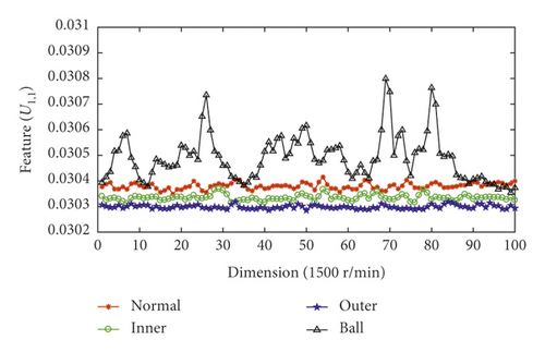
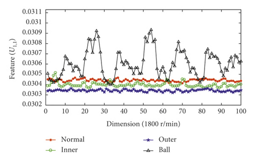
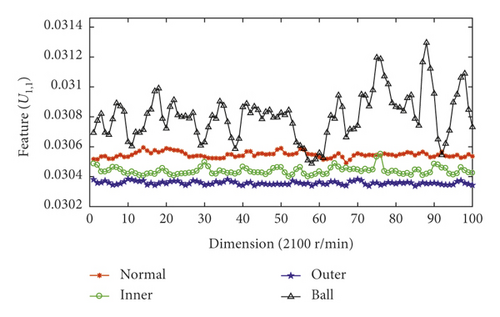
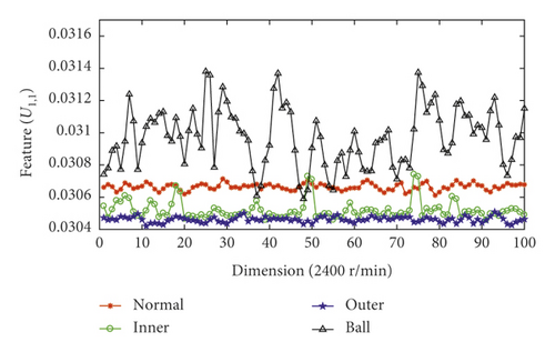
In this experiment, v = 100 and σ = 200. 100 groups of feature samples were extracted for the normal bearing to form a dataset with dimensions of 8 × 100; comparatively, the dataset matrix with dimensions of 8 × 100 of each bearing (inner ring fault, outer ring fault, and ball fault) was also extracted.

Figure 4 shows the fault feature vector corresponding to sensor 1 at different rotating speeds. As shown, the proposed VMD fault feature method better represents different fault information.

5.3. Model Optimization and Performance Analysis

Fifty groups of samples were selected from each fault sample dataset (normal, inner ring, outer ring, and ball fault bearings) to construct the training sample matrix with dimensions of 8 × 200; the remaining samples of each fault bearing dataset were used to construct the testing sample matrix with dimensions of 8 × 200. The parameters Gaussian kernel function σ and penalty factor C greatly influence diagnostic accuracy; given this, when the EALO algorithm was used for optimal parameter selection, the searching space range was defined as 2⁻⁵ < σ < 2¹⁰ and 2⁰ < C < 2³⁰.

To verify the effectiveness of the EALO method proposed here, the ALO, genetic algorithm (GA), and particle swarm optimization (PSO) methods with different parameters were selected for comparison. All algorithms were executed on a computer running Windows 10 ×64 operating system with an Intel® Core™ i7-8700k [email protected] GHz and with a memory capacity of 64 GB. To prevent the algorithms from iterating indefinitely, the maximum number of iterations I_ter = 100 was adopted. Additional parameters for different algorithms are shown in Table 2.

Table 2. Details of different algorithm parameters.

Algorithm	Searching range	Convergence condition	Parameter	Initial value
EALO	2⁻⁵ < σ < 2¹⁰ 2⁰ < C < 2³⁰	ε = 10⁻⁶	Ant population	50
			Ant lion population	25
			Escape ant population	10
			Ant escape probability	0.7

ALO	2⁻⁵ < σ < 2¹⁰ 2⁰ < C < 2³⁰	I_ter = 100	Ant population	50
ALO	2⁻⁵ < σ < 2¹⁰ 2⁰ < C < 2³⁰	I_ter = 100	Ant lion population	25

GA-1	2⁻⁵ < σ < 2¹⁰ 2⁰ < C < 2³⁰	ε = 10⁻⁶ \|\| I_ter = 100	Population	50
			Crossover probability	0.1
			Mutation probability	0.01

GA-2	2⁻⁵ < σ < 2¹⁰ 2⁰ < C < 2³⁰	ε = 10⁻⁶ \|\| I_ter = 100	Population	50
			Crossover probability	0.4
			Mutation probability	0.01

GA-3	2⁻⁵ < σ < 2¹⁰ 2⁰ < C < 2³⁰	ε = 10⁻⁶ \|\| I_ter = 100	Population	50
			Crossover probability	0.1
			Mutation probability	0.1

GA-4	2⁻⁵ < σ < 2¹⁰ 2⁰ < C < 2³⁰	ε = 10⁻⁶ \|\| I_ter = 100	Population	50
			Crossover probability	0.4
			Mutation probability	0.1

GA-5	2⁻⁵ < σ < 2¹⁰ 2⁰ < C < 2³⁰	ε = 10⁻⁶ \|\| I_ter = 100	Population	50
			Crossover probability	0.7
			Mutation probability	0.5

PSO-1	2⁻⁵ < σ < 2¹⁰ 2⁰ < C < 2³⁰	ε = 10⁻⁶ \|\| I_ter = 100	Particle size	50
			Acceleration factor C1	0.1
			Acceleration factor C2	0.1
			Weight W	0.5

PSO-2	2⁻⁵ < σ < 2¹⁰ 2⁰ < C < 2³⁰	ε = 10⁻⁶ \|\| I_ter = 100	Particle size	50
			Acceleration factor C1	0.5
			Acceleration factor C2	0.1
			Weight W	0.8

PSO-3	2⁻⁵ < σ < 2¹⁰ 2⁰ < C < 2³⁰	ε = 10⁻⁶ \|\| I_ter = 100	Particle size	50
			Particle size	1.0
			Acceleration factor C1	0.5
			Acceleration factor C2	1.0
			Weight W	100

PSO-4	2⁻⁵ < σ < 2¹⁰ 2⁰ < C < 2³⁰	ε = 10⁻⁶ \|\| I_ter = 100	Particle size	50
			Acceleration factor C1	1.5
			Acceleration factor C2	1.7
			Weight W	1.0

PSO-5	2⁻⁵ < σ < 2¹⁰ 2⁰ < C < 2³⁰	ε = 10⁻⁶ \|\| I_ter = 100	Particle size	50
			Acceleration factor C1	2.0
			Acceleration factor C2	2.0
			Weight W	1.5

Using the rotation speed of 1500 r/min as an example, the distributional status of the ant and ant lion populations in the SVM parameter optimization processed by EALO is shown in Figure 5. As shown, as the iteration number increased, the ant and ant lion populations gradually converged to the optimal solution region, indicating that the EALO algorithm was convergent. As shown in Figure 5(a), the initial distributions of the ant and ant lion populations are randomly distributed. The ant lions build traps at random initial locations to prepare for the later capture of ants.

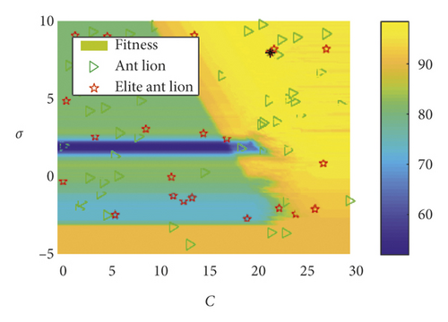
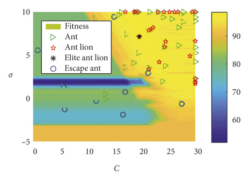
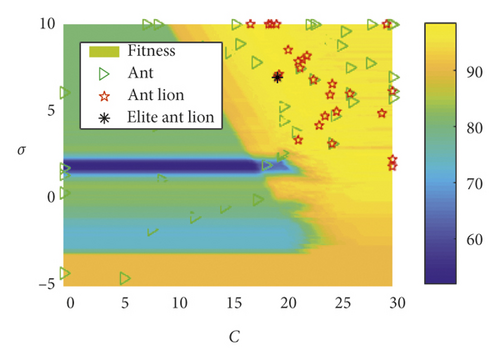
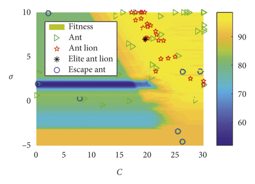
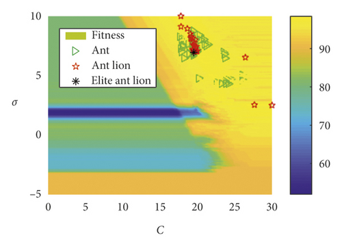
When considering the escape mechanism, there is a given probability that some ants will escape the trap of an ant lion. As shown in Figure 5, when the EALO iterates for the third (Figure 5(b)), seventh (Figure 5(d)), and ninth (Figure 5(e)) times, some of the ants exit the ant lion’s trap and escape to other random locations (labeled “o”). Therefore, the probability that the algorithm falls into local extremum is effectively reduced, and the overall optimization performance of the algorithm is improved. It can also be seen from Figure 5 that the kernel function parameter σ and the penalty factor C greatly influenced the accuracy of the bearing fault classification. When the EALO algorithm stopped iteration (Figure 5(f)), the ant and ant lion locations did not converge to a single point. Rather, these locations converged to multiple points, which demonstrated that there were multiple feasible solutions. Therefore, any ant lion could be selected as the elite ant lion, and its position is regarded as the optimal algorithm solution.

Using bearing fault diagnosis at a speed of 1500 r/min as an example, the convergence curves for EALO, ALO, GA, and PSO are all shown in Figure 6. As shown, the EALO method iterates only 13 times, while the ALO, GA, and PSO iterate 100 times. Although threshold conditions were satisfied after 70 iterations, the ALO method did not stop iterating because it did not have an escape mechanism or adaptive convergence condition. During iteration, if the ants walk around the poor fitness ant lions, the probability of falling into local extremum is increased; simultaneously, the resources of the ant lion individual will be wasted owing to the ant lion’s search in the local extremum neighborhood. Therefore, the optimization performance and the convergence efficiency of the ALO algorithm is partly reduced. The threshold values for the EALO and ALO methods gradually decrease with increasing iteration time.

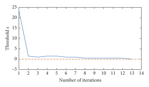
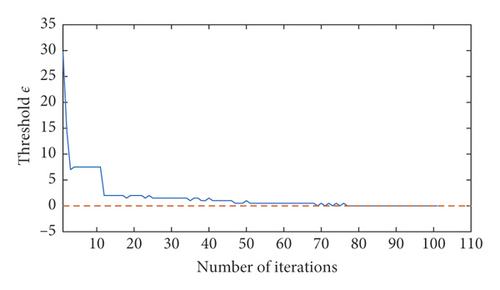
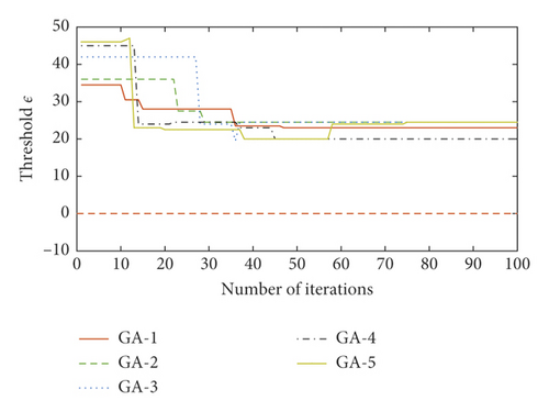
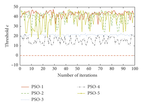
Using different parameters, the convergence performance of the GA method is different. Using inappropriate parameters resulted in GA performance deterioration; as shown in GA-5, the performance threshold ε increased with 60 iteration times and no longer decreased after a certain number of iterations. Finally, the PSO optimization performance was also greatly affected by its attendant parameters. The PSO iterative curve oscillated and had no obvious convergence trend, indicating that the convergence condition proposed here was not suitable for the PSO method. Taken together, these findings show that the EALO method proposed here had the fastest convergence speed.

5.4. Results and Discussion

It has been reported that the binary tree model is a more suitable approach to classify bearing faults than many other classification models [19]. This is because the radial basis kernel function has better nonlinear mapping ability in high-dimensional space than other kernel functions, making this model better suited for the fault classification of bearings. Therefore, both the binary tree support vector machine model and the radial basis kernel function model were used in these experiments. The EALO, traditional ALO, GA, and PSO methods with different parameters were used to optimize the SVM model parameters. Four faults of bearings at different speeds were then diagnosed by this optimized SVM model. The diagnostic results are shown in Tables 3–6.

Table 3. Model optimization and bearing fault diagnostic results at 1500 r/min.

Methods	Log₂(C^∗)	Log₂(σ^∗)	Time (s)	Iteration number	SV number	Testing dataset		Training dataset
Methods	Log₂(C^∗)	Log₂(σ^∗)	Time (s)	Iteration number	SV number	Faults	Recognition rate (%)	Faults	Recognition rate (%)
EALO	19.5487	6.9794	0.9065	13	62	Normal	100	Normal	100
						Inner	100	Inner	96
						Outer	100	Outer	100
						Ball	98	Ball	100
						Average	99.5	Average	99
						Total average		99.25

ALO	18.5233	8.3764	4.6771	100	59	Normal	100	Normal	100
						Inner	94	Inner	94
						Outer	100	Outer	100
						Ball	98	Ball	98
						Average	98	Average	98
						Total average		98

GA-1	27.9121	2.4963	9.7142	100	43	Normal	92	Normal	100
						Inner	90	Inner	88
						Outer	100	Outer	100
						Ball	98	Ball	98
						Average	95	Average	96.5
						Total average		95.75

GA-2	18.2271	9.5530	9.6264	100	48	Normal	100	Normal	100
						Inner	94	Inner	96
						Outer	100	Outer	100
						Ball	98	Ball	98
						Average	98	Average	98.5
						Total average		98.25

GA-3	20.0440	9.1353	9.9713	100	34	Normal	100	Normal	100
						Inner	94	Inner	96
						Outer	100	Outer	100
						Ball	100	Ball	98
						Average	98.5	Average	98.5
						Total average		98.5

GA-4	17.7436	4.6214	10.9412	100	163	Normal	100	Normal	100
						Inner	94	Inner	90
						Outer	100	Outer	100
						Ball	94	Ball	86
						Average	97	Average	94
						Total average		95.5

GA-5	10.6886	-2.4792	10.3611	100	200	Normal	100	Normal	100
						Inner	92	Inner	88
						Outer	100	Outer	100
						Ball	0	Ball	4
						Average	73	Average	73
						Total average		73

PSO-1	22.3069	5.9467	10.6698	100	41	Normal	100	Normal	100
						Inner	92	Inner	96
						Outer	100	Outer	100
						Ball	98	Ball	98
						Average	97.5	Average	98.5
						Total average		98

PSO-2	30.0000	2.5238	9.1010	100	47	Normal	52	Normal	68
						Inner	92	Inner	98
						Outer	100	Outer	100
						Ball	98	Ball	98
						Average	85.5	Average	91
						Total average		88.25

PSO-3	30.0000	9.8034	8.9303	100	171	Normal	96	Normal	98
						Inner	72	Inner	78
						Outer	98	Outer	100
						Ball	82	Ball	70
						Average	87	Average	86.5
						Total average		86.75

PSO-4	19.0039	8.0955	8.3374	100	56	Normal	100	Normal	100
						Inner	94	Inner	9
						Outer	100	Outer	100
						Ball	98	Ball	98
						Average	98	Average	98
						Total average		98

PSO-5	10.8694	-1.9647	8.8360	100	200	Normal	96	Normal	98
						Inner	72	Inner	78
						Outer	98	Outer	100
						Ball	50	Ball	46
						Average	79	Average	80.5
						Total average		79.75

Table 4. Model optimization and bearing fault diagnostic results at 1800 r/min.

Methods	Log₂(C^∗)	Log₂(σ^∗)	Time (s)	Iteration number	SV number	Testing dataset		Training dataset
Methods	Log₂(C^∗)	Log₂(σ^∗)	Time (s)	Iteration number	SV number	Faults	Recognition rate (%)	Faults	Recognition rate (%)
EALO	23.7849	3.8057	0.9349	15	20	Normal	100	Normal	98
						Inner	100	Inner	100
						Outer	100	Outer	100
						Ball	98	Ball	100
						Average	99.5	Average	99.5
						Total average		99.5

ALO	19.8388	8.68205	4.3750	100	33	Normal	100	Normal	98
						Inner	100	Inner	96
						Outer	100	Outer	100
						Ball	98	Ball	100
						Average	99.5	Average	98.5
						Total average		99

GA-1	22.8205	5.7719	9.1252	100	29	Normal	100	Normal	98
						Inner	100	Inner	98
						Outer	100	Outer	100
						Ball	98	Ball	100
						Average	99.5	Average	99
						Total average		99.25

GA-2	23.9121	7.6404	10.4754	100	18	Normal	100	Normal	98
						Inner	100	Inner	96
						Outer	100	Outer	100
						Ball	100	Ball	100
						Average	100	Average	98.5
						Total average		99

GA-3	27.8681	6.7904	10.6654	100	21	Normal	100	Normal	98
						Inner	100	Inner	96
						Outer	100	Outer	100
						Ball	100	Ball	100
						Average	100	Average	98.5
						Total average		99.25

GA-4	19.9341	-4.3258	9.4085	100	200	Normal	100	Normal	100
						Inner	92	Inner	88
						Outer	100	Outer	100
						Ball	44	Ball	68
						Average	84	Average	89
						Total average		86.5

GA-5	19.5385	9.28187	10.6452	100	30	Normal	100	Normal	98
						Inner	100	Inner	96
						Outer	100	Outer	100
						Ball	98	Ball	100
						Average	99.5	Average	98.5
						Total average		99

PSO-1	20.0281	8.3309	8.4335	100	32	Normal	100	Normal	100
						Inner	100	Inner	96
						Outer	100	Outer	100
						Ball	98	Ball	100
						Average	99.5	Average	99
						Total average		99.25

PSO-2	18.5136	10.0000	8.9782	100	31	Normal	100	Normal	98
						Inner	100	Inner	96
						Outer	100	Outer	100
						Ball	98	Ball	100
						Average	99.5	Average	98.5
						Total average		99

PSO-3	28.0514	7.4172	8.0311	100	22	Normal	100	Normal	98
						Inner	100	Inner	98
						Outer	100	Outer	100
						Ball	100	Ball	100
						Average	100	Average	99
						Total average		99.5

PSO-4	18.6287	10.0000	8.0532	100	31	Normal	100	Normal	98
						Inner	100	Inner	96
						Outer	100	Outer	100
						Ball	98	Ball	100
						Average	99.5	Average	98.5
						Total average		99

PSO-5	18.4047	10.0000	7.5552	100	31	Normal	100	Normal	98
						Inner	100	Inner	96
						Outer	100	Outer	100
						Ball	98	Ball	100
						Average	99.5	Average	98.5
						Total average		99

Table 5. Model optimization and bearing fault diagnostic results at 2100 r/min.

Methods	Log₂(C^∗)	Log₂(σ^∗)	Time (s)	Iteration number	SV number	Testing dataset		Training dataset
Methods	Log₂(C^∗)	Log₂(σ^∗)	Time (s)	Iteration number	SV number	Faults	Recognition rate (%)	Faults	Recognition rate (%)
EALO	23.2934	7.6761	0.2366	3	19	Normal	100	Normal	100
						Inner	100	Inner	98
						Outer	100	Outer	100
						Ball	100	Ball	98
						Average	100	Average	99
						Total average		99.5

ALO	25.7334	7.2869	3.3147	100	20	Normal	100	Normal	100
						Inner	100	Inner	98
						Outer	100	Outer	100
						Ball	100	Ball	98
						Average	100	Average	99
						Total average		99.5

GA-1	25.4725	5.1417	7.4716	100	22	Normal	100	Normal	100
						Inner	100	Inner	98
						Outer	100	Outer	100
						Ball	100	Ball	98
						Average	100	Average	99
						Total average		99.5

GA-2	29.2674	4.5188	11.8305	100	17	Normal	100	Normal	100
						Inner	100	Inner	98
						Outer	100	Outer	100
						Ball	100	Ball	98
						Average	100	Average	99
						Total average		99.5

GA-3	28.7179	9.4871	9.7435	100	20	Normal	100	Normal	100
						Inner	100	Inner	98
						Outer	100	Outer	100
						Ball	100	Ball	98
						Average	100	Average	99
						Total average		99.5

GA-4	20.1026	9.2599	8.0058	100	19	Normal	100	Normal	100
						Inner	100	Inner	98
						Outer	100	Outer	100
						Ball	100	Ball	98
						Average	100	Average	99
						Total average		99.5

GA-5	13.0549	8.0581	8.5892	100	139	Normal	100	Normal	98
						Inner	98	Inner	96
						Outer	100	Outer	100
						Ball	100	Ball	100
						Average	99.5	Average	98
						Total average		99

PSO-1	27.0491	5.2417	8.8048	100	19	Normal	100	Normal	100
						Inner	100	Inner	98
						Outer	100	Outer	100
						Ball	100	Ball	98
						Average	100	Average	99
						Total average		99.5

PSO-2	15.4353	10.0000	8.2438	100	32	Normal	100	Normal	100
						Inner	100	Inner	96
						Outer	100	Outer	100
						Ball	100	Ball	98
						Average	100	Average	98.5
						Total average		99.25

PSO-3	18.4043	9.0937	7.7971	100	22	Normal	100	Normal	100
						Inner	100	Inner	98
						Outer	100	Outer	100
						Ball	100	Ball	98
						Average	100	Average	99
						Total average		99.5

PSO-4	20.3913	10.0000	7.7289	100	20	Normal	100	Normal	100
						Inner	100	Inner	98
						Outer	100	Outer	100
						Ball	100	Ball	98
						Average	100	Average	99
						Total average		99.5

PSO-5	30.0000	9.8561	5.8882	100	19	Normal	100	Normal	100
						Inner	100	Inner	98
						Outer	100	Outer	100
						Ball	100	Ball	98
						Average	100	Average	99
						Total average		99.5

Table 6. Model optimization and bearing fault diagnostic results at 2400 r/min.

Methods	Log₂(C^∗)	Log₂(σ^∗)	Time (s)	Iteration number	SV number	Testing dataset		Training dataset
Methods	Log₂(C^∗)	Log₂(σ^∗)	Time (s)	Iteration number	SV number	Faults	Recognition rate (%)	Faults	Recognition rate (%)
EALO	26.5027	6.4664	0.2656	3	22	Normal	100	Normal	100
						Inner	100	Inner	98
						Outer	100	Outer	100
						Ball	100	Ball	100
						Average	100	Average	99.5
						Total average		99.75

ALO	30.0000	1.7908	3.4479	100	27	Normal	94	Normal	88
						Inner	100	Inner	100
						Outer	100	Outer	100
						Ball	100	Ball	100
						Average	98.5	Average	97
						Total average		97.75

GA-1	24.4322	5.4787	9.9083	100	21	Normal	100	Normal	100
						Inner	100	Inner	98
						Outer	100	Outer	100
						Ball	100	Ball	100
						Average	100	Average	99.5
						Total average		99.75

GA-2	23.2381	7.7137	10.2449	100	22	Normal	100	Normal	100
						Inner	100	Inner	98
						Outer	100	Outer	100
						Ball	100	Ball	100
						Average	100	Average	99.5
						Total average		99.75

GA-3	21.7289	8.6957	9.1041	100	23	Normal	100	Normal	100
						Inner	100	Inner	98
						Outer	100	Outer	100
						Ball	100	Ball	100
						Average	100	Average	99.5
						Total average		99.75

GA-4	22.4615	6.4680	8.4840	100	22	Normal	100	Normal	100
						Inner	100	Inner	98
						Outer	100	Outer	100
						Ball	100	Ball	100
						Average	100	Average	99.5
						Total average		99.75

GA-5	24.9011	9.3258	10.8618	100	24	Normal	100	Normal	100
						Inner	100	Inner	98
						Outer	100	Outer	100
						Ball	100	Ball	100
						Average	100	Average	99.5
						Total average		99.75

PSO-1	30.0000	1.8006	6.9233	100	26	Normal	88	Normal	84
						Inner	100	Inner	100
						Outer	100	Outer	100
						Ball	100	Ball	100
						Average	97	Average	96
						Total average		96.5

PSO-2	30.0000	1.7888	8.8493	100	27	Normal	92	Normal	88
						Inner	100	Inner	100
						Outer	100	Outer	100
						Ball	100	Ball	100
						Average	98	Average	97
						Total average		97.5

PSO-3	30.0000	1.88131	7.6882	100	29	Normal	100	Normal	100
						Inner	100	Inner	96
						Outer	100	Outer	100
						Ball	100	Ball	100
						Average	100	Average	99
						Total average		99.5

PSO-4	30.0000	7.4530	6.5468	100	24	Normal	100	Normal	100
						Inner	100	Inner	98
						Outer	100	Outer	100
						Ball	100	Ball	100
						Average	100	Average	99.5
						Total average		99.75

PSO-5	20.5845	9.0898	7.2608	100	23	Normal	100	Normal	100
						Inner	100	Inner	98
						Outer	100	Outer	100
						Ball	100	Ball	100
						Average	100	Average	99.5
						Total average		99.75

As shown in Table 3, when the rotation speed was 1500 r/min, the number of EALO iterations proposed here was 13. Moreover, the optimization time was the shortest (0.9065 s), followed by the ALO approach (4.6771 s). The GA approach took the longest (9.6264 s). The same results were found when the rotation speeds were 1800 r/min (Table 4), 2100 r/min (Table 5), and 2400 r/min (Table 6). The reasons for these results are that the GA method requires a series of operations (e.g., encoding, selection, crossover, mutation, and decoding), resulting in a complex genetic algorithm. Contrastingly, the interaction between ants and ant lions in the EALO did not require complex operations. Additionally, the escape mechanism and effective adaptive convergence conditions were introduced, which greatly reduced the number of iterations and improved its optimization performance. In the PSO, particle velocity and direction were controlled by many parameters, including the acceleration factors C₁ and C₂ as well as the inertia weight W; these parameters had greater influence on PSO algorithm convergence with improper parameters resulting in the algorithm falling into the local extremum. Optimal parameters are difficult to obtain in practice, and as a result, it was difficult for the particles to converge. Ultimately, this reduced the PSO’s performance.

Table 7 details the support vector (SV) number of the SVM model optimized by different methods at different speeds. When compared with the complexity of the optimized SVM model, the total average number of SVs of the SVM model optimized by the EALO was 23; notably, this was the least average number. Comparatively, the total average number of ALO, PSO, and GA support vectors was 34.75, 45.15, and 55.75, respectively. To some extent, the SV number represents the complexity of the high-dimensional space of the SVM model—the lower the SV number, the higher the linear separability in the high-dimensional space. Taken together, the results presented here show that the kernel function parameters and penalty factors optimized by the improved EALO method allow the kernel function to have greater nonlinear mapping ability.

Table 7. SV number of the SVM model optimized by different methods at different speeds.

Methods	SV number				Average SV number	Total average SV number
Methods	1500 r/min	1800 r/min	2100 r/min	2400 r/min	Average SV number	Total average SV number
EALO	31	20	19	22	—	23.00
ALO	59	33	20	27	—	34.75
GA-1	43	29	22	21	28.75	55.75
GA-2	48	18	17	22	26.25
GA-3	34	21	20	23	24.5
GA-4	163	200	19	22	101
GA-5	200	30	139	24	98.25
PSO-1	41	32	19	26	29.5	45.15
PSO-2	47	31	32	27	34.25
PSO-3	171	22	22	29	61
PSO-4	56	31	20	24	32.75
PSO-5	200	31	19	23	68.25

The average bearing fault recognition rates using different optimization methods (e.g., EALO, ALO, GA, and PSO) at different speeds are shown in Table 8. As shown, the EALO method proposed here achieved the highest recognition accuracy (99.5%) using the four rotation speeds. This was followed by the ALO, GA, and PSO methods, which had accuracies of 98.56%, 96.99%, and 96.84%, respectively. These findings show that the EALO method proposed here has better optimization ability than the other three methods. Moreover, the optimized parameters were closer to the real optimal solution. Therefore, these results show that the improved EALO method can effectively improve the recognition rate of bearing faults.

Table 8. Average recognition rate of bearing faults using four optimization methods at different speeds.

Methods	Recognition rate (%)				Average recognition rate (%)	Total average recognition rate (%)
Methods	1500 r/min	1800 r/min	2100 r/min	2400 r/min	Average recognition rate (%)	Total average recognition rate (%)
EALO	99.25	99.50	99.50	99.75	—	99.50
ALO	98.00	99.00	99.50	97.75	—	98.56
GA-1	95.75	99.25	99.50	99.75	98.56	96.99
GA-2	98.25	99.00	99.50	99.75	99.13
GA-3	98.50	99.25	99.50	99.75	99.25
GA-4	95.50	86.50	99.50	99.75	95.31
GA-5	73.00	99.00	99.00	99.75	92.69
PSO-1	98.00	99.25	99.50	96.50	98.31	96.84
PSO-2	88.25	99.00	99.25	97.50	96.00
PSO-3	86.75	99.50	99.50	99.50	96.31
PSO-4	98.00	99.00	99.50	99.75	99.06
PSO-5	79.75	99.00	99.50	99.75	94.50

6. Conclusion

Based on the classical ALO algorithm, the EALO algorithm was proposed by introducing an escape mechanism and adaptive iterative convergence conditions. This algorithm was then applied to the diagnosis of bearing faults. Comparing with more traditional methods (e.g., ALO, GA, and PSO), the following conclusions can be drawn:

(1)
The escape mechanism was effective and reduced the possibility that the classical ALO algorithm would fall into a local extremum value. This improved the global optimization performance.
(2)
The proposed adaptive convergence conditions effectively reduced the iteration number, saving optimization time and improving the optimization performance of the EALO algorithm.
(3)
The proposed EALO algorithm was suitable for SVM parameter optimization. When compared with the classical ALO, GA, and PSO approaches, the EALO algorithm had the best performance.
(4)
The feature extraction method based on the VMD and kernel function was effective and provides a new reference point for bearing fault diagnosis.

Conflicts of Interest

The authors declare that they have no conflicts of interest.

Acknowledgments

This study was supported by the National Natural Science Foundation of China (Grant Nos. 11702091 and 51575178), the Natural Science Foundation of Hunan Province of China (Grant Nos. 2018JJ3140, 2019JJ50156, and 2018JJ4084), Hunan Provincial Key Research and Development Program (Grant No. 2018GK2044), and Open Funded Projects of Hunan Provincial Key Laboratory of Health Maintenance for Mechanical Equipment (Grant No. 201605).

Open Research

Data Availability

The data used to support the findings of this study are included in the supplementary file “Datasets.zip.”

Supporting Information

References

1 Cui L., Huang J., and Zhang F., Quantitative and localization diagnosis of a defective ball bearing based on vertical-horizontal synchronization signal analysis, IEEE Transactions on Industrial Electronics. (2017) 64, no. 11, 8695–8706, https://doi.org/10.1109/tie.2017.2698359, 2-s2.0-85035767656.
10.1109/TIE.2017.2698359
Web of Science® Google Scholar
2 Gao Q., Tang H., Xiang J., Zhong Y., Ye S., and Pang J., A Walsh transform-based teager energy operator demodulation method to detect faults in axial piston pumps, Measurement. (2019) 134, 293–306, https://doi.org/10.1016/j.measurement.2018.10.085, 2-s2.0-85055712600.
10.1016/j.measurement.2018.10.085
Web of Science® Google Scholar
3 Tao J., Liu Y., and Yang D., Bearing fault diagnosis based on deep belief network and multisensor information fusion, Shock and Vibration. (2016) 2016, 1–9, https://doi.org/10.1155/2016/9306205, 2-s2.0-84988735586.
10.1155/2016/9306205
Web of Science® Google Scholar
4 Taylor J. I., Back to the basics of the rotating machinery vibration analysis, Sound and Vibration. (1995) 29, no. 2, 12–16.
Web of Science® Google Scholar
5 Wang L. and Xiang J., A two-stage method using spline-kernelled chirplet transform and angle synchronous averaging to detect faults at variable speed, IEEE Access. (2019) 7, no. 1, 22471–22485, https://doi.org/10.1109/access.2019.2898884, 2-s2.0-85062939249.
10.1109/ACCESS.2019.2898884
Web of Science® Google Scholar
6 Li X., Jiang L., Yang D., and Wang K., Cluster analysis and fault diagnosis for gear based on bispectrum distribution, Journal of Vibration Engineering. (2011) 3, no. 24, 304–308.
Google Scholar
7 Wang S., Xiang J., Zhong Y., and Tang H., A data indicator-based deep belief networks to detect multiple faults in axial piston pumps, Mechanical Systems and Signal Processing. (2018) 112, 154–170, https://doi.org/10.1016/j.ymssp.2018.04.038, 2-s2.0-85046339195.
10.1016/j.ymssp.2018.04.038
Web of Science® Google Scholar
8 Saravanan N. and Ramachandran K. I., Incipient gear box fault diagnosis using discrete wavelet transform (DWT) for feature extraction and classification using artificial neural network (ANN), Expert Systems with Applications. (2010) 37, no. 6, 4168–4181, https://doi.org/10.1016/j.eswa.2009.11.006, 2-s2.0-77349127319.
10.1016/j.eswa.2009.11.006
Web of Science® Google Scholar
9 Samanta B. and Al-Balushi K. R., Artificial neural network based fault diagnostics of rolling element bearings using time-domain features, Mechanical Systems and Signal Processing. (2003) 17, no. 2, 317–328, https://doi.org/10.1006/mssp.2001.1462, 2-s2.0-0037345899.
10.1006/mssp.2001.1462
Web of Science® Google Scholar
10 Zhu Y., Huo L., and Lu J., Bayesian networks-based approach for power systems fault diagnosis, IEEE Transactions on Power Delivery. (2006) 21, no. 2, 634–639, https://doi.org/10.1109/tpwrd.2005.858774, 2-s2.0-33645741993.
10.1109/TPWRD.2005.858774
Web of Science® Google Scholar
11 Wang C. C., Kang Y., and Liao C. C., Using bayesian networks in gear fault diagnosis, Applied Mechanics and Materials. (2013) 284-287, no. 287, 2416–2420, https://doi.org/10.4028/www.scientific.net/amm.284-287.2416, 2-s2.0-84873927784.
10.4028/www.scientific.net/AMM.284-287.2416
Google Scholar
12 Jiang R., Yu J., and Makis V., Optimal Bayesian estimation and control scheme for gear shaft fault detection, Computers and Industrial Engineering. (2012) 63, no. 4, 754–762, https://doi.org/10.1016/j.cie.2012.04.015, 2-s2.0-84868203717.
10.1016/j.cie.2012.04.015
Web of Science® Google Scholar
13 Cortes C. and Vapnik V., Support vector machine, Machine learning. (1995) 20, no. 3, 273–297, https://doi.org/10.1007/bf00994018.
10.1007/BF00994018
Web of Science® Google Scholar
14 Xiang J. and Zhong Y., A novel personalized diagnosis methodology using numerical simulation and an intelligent method to detect faults in a shaft, Applied Sciences. (2016) 6, no. 12, https://doi.org/10.3390/app6120414, 2-s2.0-85007451868.
10.3390/app6120414
Google Scholar
15 Samanta B., Gear fault detection using artificial neural networks and support vector machines with genetic algorithms, Mechanical Systems and Signal Processing. (2004) 18, no. 3, 625–644, https://doi.org/10.1016/s0888-3270(03)00020-7, 2-s2.0-0942289503.
10.1016/S0888-3270(03)00020-7
Web of Science® Google Scholar
16 Joachims T., B. C. J. Schölkopf and A. Smola, Making Large-Scale SVM learning practical, Advances in Kernel Methods-Support Vector Learning, 1998, MIT Press, Cambridge, MA, USA, 169–184.
10.7551/mitpress/1130.003.0015
Google Scholar
17 Yang Y. and Pederson J. O., A comparative study on feature selection in text categorization, Proceedings of the 14th International Conference on Machine Learning, July 1997, Nashville, TN, USA, Morgan Kaufmann, 412–420.
Google Scholar
18 Drucker H., Burges C. J., Kaufman L., Smola A., and Vapnik V., M. Mozer, M. Jordan, and T. Petsche, Support vector regression machines, Neural Information Processing Systems, 1997, 9, MIT Press, Cambridge, MA, USA.
Google Scholar
19 Guyon L., Matic N., and Vapnik V., Discovering Information Pattern and Data Cleaning, 1997, AT&T Bell Laboratory, Murray Hill, NJ, USA.
Google Scholar
20 Jiang L., Liu Y., Li X., and Chen A., Gear fault diagnosis based on SVM and multi-sensor information fusion, Journal of Central South University (Science and Technology). (2010) 6, 2184–2188.
Google Scholar
21 Li X., Yang D., Guo D., and Jiang L., Fault diagnosis method based on multi-sensors installed on the base and KPCA, Chinese Journal of Scientific Instrument. (2011) 7, 1551–1557.
Google Scholar
22 Liu Q., Chen G., Liu X., and Yang Q., Genetic algorithm based SVM parameter composition optimization, Computer Applications and Software. (2012) 4, 94–96.
Google Scholar
23 Cheng H., Huang C., and Zhang Y., Constructed of SVM decision tree based on particle swarm optimization algorithm for gear box fault diagnosis, Journal of Vibration, Measurement and Diagnosis. (2013) 1, 153–156.
Google Scholar
24 Yang D., Liu Y., Li S., Li X., and Ma L., Gear fault diagnosis based on support vector machine optimized by artificial bee colony algorithm, Mechanism and Machine Theory. (2015) 90, no. 3, 219–229, https://doi.org/10.1016/j.mechmachtheory.2015.03.013, 2-s2.0-84927621097.
10.1016/j.mechmachtheory.2015.03.013
Web of Science® Google Scholar
25 Mirjalili S., The ant lion optimizer, Advances in Engineering Software. (2015) 83, 80–98, https://doi.org/10.1016/j.advengsoft.2015.01.010, 2-s2.0-84923355494.
10.1016/j.advengsoft.2015.01.010
Web of Science® Google Scholar
26 Wu W., Zhang J., Lin Z., and Su Q., Ant lion optimization algorithm based on double feedback mechanism, Computer Engineering and Applications. (2017) 53, no. 12, 31–35.
Google Scholar
27 Jing K., Zhao X., Zhang X., and Liu D., Ant lion optimizer with levy variation and adaptive elite competition mechanisms, CAAI Transactions on Intelligent Systems. (2018) 2, 1–8.
Google Scholar
28 Talatahari S., Optimum design of skeletal structures using ant lion optimizer, International Journal of Optimization in Civil Engineering. (2016) 6, no. 1, 3–25.
Google Scholar
29 Saxena P. and Kothari A., Ant Lion Optimization algorithm to control side lobe level and null depths in linear antenna arrays, AEU-International Journal of Electronics and Communications. (2016) 70, no. 9, 1339–1349, https://doi.org/10.1016/j.aeue.2016.07.008, 2-s2.0-84978864833.
10.1016/j.aeue.2016.07.008
Web of Science® Google Scholar
30 Mohammad J. H. M., Saber A. N., and Mehdi B., A multi-objective optimal Sizing and siting of distributed generation using ant lion optimization technique, Ain Shams Engineering Journal. (2017) 9, no. 4, 2101–2109, https://doi.org/10.1016/j.asej.2017.03.001, 2-s2.0-85019732035.
10.1016/j.asej.2017.03.001
Web of Science® Google Scholar
31 Mei R. G. S., Sulaiman M. H., and Mustaffa A., Ant lion optimizer for optimal reactive power dispatch solution, Journal of Electrical Systems. (2015) 3, 67–74.
Google Scholar
32 Mahajan A. and Kaur M. G., Community Detection in Complex Networks Using a Novel Nature Inspired Algorithmic Approach based on Ant Lion Optimizer, 2015, Thapar University Patiala, Patiala, India.
Google Scholar
33 Zhong Y., Zha J., and Zhu S., Feature selection algorithm using Bayesian harmony measures, Computer Engineering and Applications. (2015) 51, no. 23, 125–130.
Google Scholar
34 He Z., Beijing electricity demand forecast based on ant lion optimizer GM (1,1) model, Modern Industrial Economy and Informatization. (2017) 7, no. 22, 57–60+83.
Google Scholar
35 Zhao S., Gao L., Yu D., and Tu J., Ant lion optimizer with chaotic investigation mechanism for optimizing SVM parameters, Journal of Frontiers of Computer Science and Technology. (2016) 10, no. 05, 722–731.
Google Scholar
36 Nello C. and John S. T., An Introduction to Support Vector Machine and the Kernel-based Learning Methods, 2000, Cambridge University Press, Cambridge, UK.
Google Scholar
37 Yang D., Liu Y., Li S., Tao J., Liu C., and Yi J., Fatigue crack growth prediction of 7075 aluminum alloy based on the GMSVR model optimized by the artificial bee colony algorithm, Engineering Computations. (2017) 34, no. 4, 1–21, https://doi.org/10.1108/ec-11-2015-0362, 2-s2.0-85021788325.
10.1108/EC-11-2015-0362
Web of Science® Google Scholar
38 Liu J., Liu Z., and Xiong Y., Improved multi-category support vector machines based on binary tree, Computer Engineering and Applications. (2010) 46, no. 33, 117–120.
Google Scholar
39 Konstantin D. and Dominique Z., Variational mode decomposition, IEEE Transactions on Signal Processing. (2014) 62, no. 3, 531–544, https://doi.org/10.1109/tsp.2013.2288675, 2-s2.0-84893418756.
10.1109/TSP.2013.2288675
Web of Science® Google Scholar
40 Wang Y., Markert R., Xiang J., and Zheng W., Research on variational mode decomposition and its application in detecting rub-impact fault of the rotor system, Mechanical Systems and Signal Processing. (2015) 60-61, 243–251, https://doi.org/10.1016/j.ymssp.2015.02.020, 2-s2.0-84925956911.
10.1016/j.ymssp.2015.02.020
Web of Science® Google Scholar
41 Aneesh C., Kumar S., Hisham P. M., and Soman K. P., Performance comparison of variational mode decomposition over empirical wavelet transform for the classification of power quality disturbances using support vector machine, Procedia Computer Science. (2015) 46, 372–380, https://doi.org/10.1016/j.procs.2015.02.033, 2-s2.0-84931388618.
10.1016/j.procs.2015.02.033
Google Scholar

Citing Literature

All articles

Bearing Fault Diagnosis Using a Support Vector Machine Optimized by an Improved Ant Lion Optimizer

Abstract

1. Introduction

2. Basic Algorithm Principles

2.1. Ant Lion Optimizer

2.1.1. Random Ant Walks

2.1.2. Building a Trap

2.1.3. Trapping in an Ant Lion’s Pit

2.1.4. Sliding Ants towards the Ant Lion

2.1.5. Catching Prey and Rebuilding the Pit

2.1.6. Elitism

2.2. Support Vector Machine

3. Ant Lion Optimizer Improvement

3.1. Improvement Based on the Escape Mechanism

3.2. Improvement Based on Adaptive Convergence Conditions

4. EALO-SVM Modeling

5. Experiments

5.1. Data Acquisition

5.2. Feature Extraction

5.3. Model Optimization and Performance Analysis

5.4. Results and Discussion

6. Conclusion

Conflicts of Interest

Acknowledgments

Open Research

Data Availability

Supporting Information

References

Citing Literature

Figures

References

Information

About Wiley Online Library

Help & Support

Opportunities

Connect with Wiley