Volume 2019, Issue 1 4862983

Research Article

Open Access

Wind Load and Structural Parameters Estimation from Incomplete Measurements

Huili Xue,

Huili Xue

Department of Civil and Environmental Engineering, Harbin Institute of Technology, Shenzhen 518055, China hit.edu.cn

Search for more papers by this author

Hongjun Liu,

Hongjun Liu

orcid.org/0000-0002-9604-2461

Department of Civil and Environmental Engineering, Harbin Institute of Technology, Shenzhen 518055, China hit.edu.cn

Search for more papers by this author

Huayi Peng,

Huayi Peng

Department of Civil and Environmental Engineering, Harbin Institute of Technology, Shenzhen 518055, China hit.edu.cn

Search for more papers by this author

Yin Luo,

Yin Luo

Department of Civil and Environmental Engineering, Harbin Institute of Technology, Shenzhen 518055, China hit.edu.cn

Search for more papers by this author

Kun Lin,

Corresponding Author

Kun Lin

[email protected]

orcid.org/0000-0002-3550-9443

Department of Civil and Environmental Engineering, Harbin Institute of Technology, Shenzhen 518055, China hit.edu.cn

Search for more papers by this author

Huili Xue,

Huili Xue

Department of Civil and Environmental Engineering, Harbin Institute of Technology, Shenzhen 518055, China hit.edu.cn

Search for more papers by this author

Hongjun Liu,

Hongjun Liu

orcid.org/0000-0002-9604-2461

Department of Civil and Environmental Engineering, Harbin Institute of Technology, Shenzhen 518055, China hit.edu.cn

Search for more papers by this author

Huayi Peng,

Huayi Peng

Department of Civil and Environmental Engineering, Harbin Institute of Technology, Shenzhen 518055, China hit.edu.cn

Search for more papers by this author

Yin Luo,

Yin Luo

Department of Civil and Environmental Engineering, Harbin Institute of Technology, Shenzhen 518055, China hit.edu.cn

Search for more papers by this author

Kun Lin,

Corresponding Author

Kun Lin

[email protected]

orcid.org/0000-0002-3550-9443

Department of Civil and Environmental Engineering, Harbin Institute of Technology, Shenzhen 518055, China hit.edu.cn

Search for more papers by this author

First published: 2019

https://doi.org/10.1155/2019/4862983

Citations: 9

Academic Editor: Stefano Manzoni

Share a link

Email
Wechat
Bluesky

Abstract

The extended minimum variance unbiased estimation approach can be used for joint state/parameter/input estimation based on the measured structural responses. However, it is necessary to measure the structural displacement and acceleration responses at each story for the simultaneous identification of structural parameters and unknown wind load. A novel method of identifying structural state, parameters, and unknown wind load from incomplete measurements is proposed. The estimation is performed in a modal extended minimum variance unbiased manner, based on incomplete measurements of wind-induced structural displacement and acceleration responses. The feasibility and accuracy of the proposed method are numerically validated by identifying the wind load and structural parameters on a ten-story shear building structure with incomplete measurements. The effects of crucial factors, including sampling duration and the number of measurements, are discussed. Furthermore, the practical application of the developed inverse method is evaluated based on wind tunnel testing results of a 234 m tall building structure. The results indicate that the structural state, parameters, and unknown wind load can be identified accurately using the proposed approach.

1. Introduction

Wind load is one of the main loads during the design stage of tall buildings [1, 2]. Studies show that the wind load on a tall building varies depending on the terrain condition, the shape of the building, and the surrounding buildings [3]. In most design processes, wind load is calculated according to the design code [4, 5]. However, it is difficult to calculate the time histories of wind load based on design code as the wind load design code is determined based on statistical information. Wind tunnel tests and computational fluid dynamic simulations are currently used to determine the time-varying wind load on a given structure [6, 7]. However, neither of the methods can exactly reproduce the incident turbulence and the characteristic of the surrounding buildings. Field measurement is regarded as the most accurate way of obtaining the time-varying wind load on tall buildings. However, due to the limitation of the wind load measurement technique, real-time measurement of wind load is difficult by field measurement. Compared to wind load measurement, the measurement of wind-induced displacement and acceleration responses is easier to achieve and more accurate.

In recent years, a lot of force estimation methods have been developed [8–10]. Law et al. identified wind load on a 50 m guyed mast from structural responses by regularization of the identification equation [11]. Lu and Law proposed a method for identifying unknown load using sensitivity measures of the dynamic response with respect to the input load [12]. Liu and Shepard developed a dynamic force identification approach based on the enhanced least squares approach in the frequency domain [13]. Ma et al. presented a Kalman filter method with a recursive estimator to determine the unknown excitation [14, 15]. The aforementioned approaches require that the unknown load has been generally point load acting at a specific DOF. However, wind loads acting on a building structure vary with space and time, and the methods in previous works cannot directly be used for wind load identification of building structures.

To address the aforementioned issue, Hwang et al. proposed the Kalman filtering approach in modal domain to estimate modal loads on a structure using limited measured response [16, 17]. Zhi et al. developed the Kalman filtering method and proper orthogonal decomposition technique to estimate the modal wind load on tall buildings [18, 19]. In 2007, Gillijns and Moor proposed an approach for joint input-state estimation in discrete-time dynamic system based on minimum variance unbiased solution [20]. Lourens et al. applied the method to estimate structural responses and unknown inputs in both numerical and experimental studies [21]. This method requires no assumption or prior knowledge about the unknown inputs, and it can be used for wind load identification in the physical domain [22]. Unfortunately, the aforementioned wind load estimation approaches assumed that the structural parameters are known a priori. However, for actual building structures, the structural parameters are generally determined based on the finite element model and it is difficult to calculate structural parameters exactly due to the material aging and damage in the structures.

To solve this problem, Wan et al. proposed a method called EGDF which is an extension of the unbiased minimum variance estimation for coupled state/input/parameter identification for nonlinear systems in state space [23]. Song developed the joint input-state estimation technique for joint input-state-parameter estimation based on the unscented minimum variance unbiased (UMVU) estimation method [24]. However, both EGDF and UMVU methods require that it is necessary to measure the acceleration responses at the locations where unknown inputs are applied, i.e., complete acceleration measurements at all DOFs are requested for simultaneous estimation of wind load and unknown structural parameters.

A novel method of the modal extended unbiased minimum variance estimation for joint state/parameter/wind load estimation from incomplete measurements is proposed in this study. The proposed method is able to simultaneously estimate the wind loads and structural parameters without using complete acceleration measurements. Moreover, the data fusion of acceleration responses and interstory displacement responses is used to prevent the drifts of the identified displacements responses and wind loads. The content of this paper is organized as follows. In Section 2, the proposed method of the modal extended unbiased minimum variance estimator is derived and the necessary mathematical proofs are given. In Section 3, a numerical validation by identifying wind loads and structural parameters from incomplete measurements on a ten-story shear building structure is addressed. Moreover, the effects of key factors, including sampling duration and the number of measurements, are discussed. In Section 4, a synchronous multipressure scanning system wind tunnel test on a 234 m tall building structure is carried out to validate the proposed method. In order to simplify the calculation, an equivalent model is carried out for experiment validation. Finally, in Section 5, the discussion and conclusion are summarized.

2. Modal Extended Minimum Variance Unbiased Estimation

2.1. System Model

The equation of motion of an n-degrees-of-freedom building structure can be written as follows:

\begin{matrix} M \ddot{x} (t) + C \dot{x} (t) + K x (t) = F (t), \end{matrix}

(1)

where M, C, and K are the n × n structural mass, damping, and stiffness matrices, respectively; F(t) is the n × 1 wind load vector;

\ddot{x} (t)

\dot{x} (t)

, and x(t) are the n × 1 wind-induced acceleration, velocity, and displacement vector, respectively.

Based on modal coordinate transformation theory [25], the structural displacement vector can be obtained as follows:

\begin{matrix} x (t) = Φ Y (t), \end{matrix}

(2)

where Φ is the n × n mass normalized modal shape matrix and Y(t) is the n × 1 modal displacement vector. By premultiplying Φ^T and using equation (2), equation (1) can be written as follows:

\begin{matrix} M_{n} {\ddot{Y}}_{n} (t) + C_{n} {\dot{Y}}_{n} (t) + K_{n} Y_{n} (t) = d_{n} (t), \end{matrix}

(3)

where M_n = Φ^TMΦ = I is the modal mass matrix, C_n = Φ^TCΦ = Γ_n is the modal damping matrix, K_n = Φ^TKΦ = Λ_n is the modal stiffness matrix, and d_n(t) = Φ^TF(t) is the modal wind load vector.

For proportionally damped system, the following can be obtained:

\begin{matrix} Γ_{n} = diag (222 ξ_{1} ω_{1}, \dots, ξ_{i} ω_{i}, \dots, ξ_{n} ω_{n}), \end{matrix}

(4)

\begin{matrix} Λ_{n} = diag (ω_{1}^{2}, \dots, ω_{i}^{2}, \dots, ω_{n}^{2}), \end{matrix}

(5)

where ω_i is the i-th undamping natural frequency and ξ_i is the i-th modal damping ratio.

Equation (3) can be rewritten as follows:

\begin{matrix} {\ddot{Y}}_{n} (t) + Γ_{n} {\dot{Y}}_{n} (t) + Λ_{n} Y_{n} (t) = d_{n} (t) . \end{matrix}

(6)

In general, due to the limitation of the number and location of the sensors, a reduced order representation of equation (6) is given:

\begin{matrix} {\ddot{Y}}_{m} (t) + Γ_{m} {\dot{Y}}_{m} (t) + Λ_{m} Y_{m} (t) = d_{m} (t), \end{matrix}

(7)

where

{\ddot{Y}}_{m} (t)

{\dot{Y}}_{m} (t)

, and Y_m(t) are the first m order modal acceleration, modal velocity, and modal displacement vector, respectively. Γ_m = diag(2ξ₁ω₁, …, 2ξ_iω_i, …, 2ξ_mω_m) and

Λ_{m} = diag (ω_{1}^{2}, \dots, ω_{i}^{2}, \dots, ω_{m}^{2})

The augmented state vector consists of the modal displacement, modal velocity, and the unknown structural parameters:

\begin{matrix} Z (t) = {[\begin{matrix} Y_{m}^{T} (t) & {\dot{Y}}_{m}^{T} (t) & θ_{p}^{T} \end{matrix}]}^{T}, \end{matrix}

(8)

where

θ_{p} = {[k_{1}, k_{2}, \dots, k_{n}, α, β]}^{T}

denotes the p × 1 unknown structural parameters vector. k_i is the i-th structural stiffness coefficient. α and β are Rayleigh damping coefficients. Assuming that the unknown structural parameters are time invariant, the first-order differential equation of equation (8) can be obtained as follows:

\begin{matrix} \dot{Z} (t) = [\begin{matrix} {\dot{Y}}_{m} (t) \\ {\ddot{Y}}_{m} (t) \\ 0 \end{matrix}] = [\begin{matrix} {\dot{Y}}_{m} (t) \\ d_{m} (t) - Γ_{m} {\dot{Y}}_{m} (t) - Λ_{m} Y_{m} (t) \\ 0 \end{matrix}] = g (Z (t), d_{m} (t)), \end{matrix}

(9)

where g(Z(t), d_m(t)) is a nonlinear function consisting of the state vector, modal wind load vector, and time t.

Denote that t_k = k × Δt with Δt as the sampling interval and define

{\overset{\land}{Z}}_{k| k}

and

{\overset{\land}{d}}_{k}

as the estimated values of Z_k and d_k at time t_k, respectively. Considering the process noise, the linearized expression of equation (9) can be expressed as follows:

\begin{matrix} g (Z_{k}, d_{k}) = g ({\overset{\land}{Z}}_{k| k}, {\overset{\land}{d}}_{k}, k Δ t) + G_{k| k}^{Z} (Z_{k} - {\overset{\land}{Z}}_{k |k}) + G_{k| k}^{d} (d_{k} - {\overset{\land}{d}}_{k}) + w_{k}, \end{matrix}

(10)

where w_k is the process noise vector with a zero mean and covariance matrix

Q_{k} = E [w_{k} w_{k}^{T}]

Furthermore, the following is obtained [26]:

\begin{matrix} G_{k| k}^{d} = {\frac{\partial g (Z_{k}, d_{k})}{\partial d_{k}}|}_{Z_{k} = {\overset{\land}{Z}}_{k| k}, d_{k} = {\overset{\land}{d}}_{k}} = [\begin{matrix} 0 \\ I \\ 0 \end{matrix}], \\ G_{k| k}^{Z} = {\frac{\partial g (Z_{k}, d_{k})}{\partial Z_{k}}|}_{Z_{k} = {\overset{\land}{Z}}_{k| k}, d_{k} = {\overset{\land}{d}}_{k}} \\ = [\begin{matrix} 0 & I & 0 \\ - Λ_{m} & - Γ_{m} & \begin{matrix} - \frac{\partial Λ_{m}}{\partial θ_{1}} Y_{m} - \frac{\partial Γ_{m}}{\partial θ_{1}} {\dot{Y}}_{m} & \dots & - \frac{\partial Λ_{m}}{\partial θ_{p}} Y_{m} - \frac{\partial Γ_{m}}{\partial θ_{p}} {\dot{Y}}_{m} \end{matrix} \\ 0 & 0 & 0 \end{matrix}] . \end{matrix}

(11)

By substituting

{\dot{Z}}_{k} = g (Z_{k}, d_{k}) = (Z_{k + 1} - Z_{k}) / (Δ t)

into the left side of equation (9), the state space equation can be obtained:

\begin{matrix} Z_{k + 1} = Z_{k} + Δ t [g ({\overset{\land}{Z}}_{k| k}, {\overset{\land}{d}}_{k}) + G_{k| k}^{Z} (Z_{k} - {\overset{\land}{Z}}_{k| k}) + G_{k| k}^{d} (d_{k} - {\overset{\land}{d}}_{k})] + Δ t \cdot w_{k} . \end{matrix}

(12)

Only the partial wind-induced displacement and acceleration responses are measured. The measurement vector is expressed as follows:

\begin{matrix} y = [\begin{matrix} x_{d} \\ {\ddot{x}}_{a} \end{matrix}], \end{matrix}

(13)

where x_d denotes d × 1 wind-induced displacement responses and

{\ddot{x}}_{a}

denotes a × 1 wind-induced acceleration responses.

Using modal coordinate transformation theory, the measurement equation at the k-th time step can be expressed as follows:

\begin{matrix} y_{k} = [\begin{matrix} Δ x_{d} \\ {\ddot{x}}_{a} \end{matrix}] \approx [\begin{matrix} D_{d} Φ_{n \times m} Y_{m} \\ D_{a} Φ_{n \times m} {\ddot{Y}}_{m} \end{matrix}] = [\begin{matrix} D_{d} Φ_{n \times m} Y_{m} \\ D_{a} Φ_{n \times m} (d_{m} - Γ_{m} {\dot{Y}}_{m} - Λ_{m} Y_{m}) \end{matrix}] = h (Z_{k}) + H_{k}^{d} d_{k}, \end{matrix}

(14)

where

Δ x_{d} = {[\begin{matrix} x_{1} & x_{2} - x_{1} & \dots & \begin{matrix} x_{n - 1} - x_{n - 2} & x_{n} - x_{n - 1} \end{matrix} \end{matrix}]}^{T}

denotes the interstory displacements, D_d is the d × n mapping matrix associated with the DOFs of the measured displacement, and D_a is the a × n mapping matrix associated with the DOFs of the measured acceleration.

Furthermore, the following is obtained:

\begin{matrix} h (Z_{k}) = [\begin{matrix} D_{d} Φ_{n \times m} Y_{m} \\ - D_{a} Φ_{n \times m} (Γ_{m} {\dot{Y}}_{m} + Λ_{m} Y_{m}) \end{matrix}], \\ H_{k}^{d} = [\begin{matrix} 0 \\ D_{a} Φ_{n \times m} d_{m} \end{matrix}] . \end{matrix}

(15)

Considering the measurement noise, the linearized measurement equation can be expressed as follows:

\begin{matrix} y_{k} = h ({\overset{\land}{Z}}_{k| k - 1}) + H_{k}^{Z} (Z_{k} - {\overset{\land}{Z}}_{k| k - 1}) + H_{k} d_{k} + v_{k}, \end{matrix}

(16)

where v_k is the measurement noise vector at the k-th time step with zero mean and covariance

R_{k} = E [v_{k} v_{k}^{T}]

Furthermore, the following is obtained:

\begin{matrix} H_{k} = [\begin{matrix} 0 \\ D_{a} Φ_{n \times m} \end{matrix}], \\ H_{k}^{Z} = [\begin{matrix} D_{d} Φ_{n \times m} & 0 & D_{d} \frac{\partial Φ_{n \times m}}{\partial θ_{1}} Y_{m} & \dots & D_{d} \frac{\partial Φ_{n \times m}}{\partial θ_{p}} Y_{m} \\ - D_{a} Φ_{n \times m} Λ_{m} & - D_{a} Φ_{n \times m} Γ_{m} & H_{k, 1}^{θ} & \dots & H_{k, i}^{θ} & \dots & H_{k, p}^{θ} \end{matrix}], \end{matrix}

(17)

where

\begin{matrix} H_{k, i}^{θ} = - D_{a} \frac{\partial Φ_{n \times m}}{\partial θ_{i}} (Γ_{m} {\dot{Y}}_{m} + Λ_{m} Y_{m}) - D_{a} Φ_{n \times m} (\frac{\partial Γ_{m}}{\partial θ_{i}} {\dot{Y}}_{m} + \frac{\partial Λ_{m}}{\partial θ_{i}} {\dot{Y}}_{m}) . \end{matrix}

(18)

2.2. Eigenvalue and Eigenvector Sensitivity

The changes in the eigenvalues and eigenvectors of the system due to changes in system parameters are used to calculate matrix

G_{k| k}^{Z}

and

H_{k}^{Z}

. For the case

θ = {[k_{1}, k_{2}, \dots, k_{n}, α, β]}^{T}

, the structural stiffness coefficient and damping coefficient are chosen as the unknown parameters. The eigenvalue problem of proportionally damped systems can be solved according to [27] as follows:

\begin{matrix} \frac{\partial λ_{l}}{\partial θ_{j}} = \frac{φ_{l}^{T} ((\partial K / \partial θ_{j}) - λ_{l} (\partial M / \partial θ_{j}))}{φ_{l}^{T} M φ_{l}}, \end{matrix}

(19)

where

λ_{l} = ω_{l}^{2}

is the l-th eigenvalue, φ_l is the l-th eigenvector, and θ_j is the j-th unknown parameter. Assuming that m modes are used for joint state-parameter-input estimation for an n-degrees-of-freedom, the eigenvector derivative can be calculated based on Wang’s method [28], as shown in the following equation:

\begin{matrix} \frac{\partial φ_{l}}{\partial θ_{j}} = \sum_{i = 1}^{m} {\bar{c}}_{i} φ_{i} + d_{l} ϖ_{l}, \end{matrix}

(20)

where

\begin{matrix} {\bar{c}}_{i} = - \frac{φ_{i}^{T} ((\partial K / \partial θ_{j}) - (\partial λ_{l} / \partial θ_{j}) M - λ_{l} (\partial M / \partial θ_{j})) φ_{l}}{λ_{i} - λ_{l}}, \\ ϖ_{l} = K^{- 1} η_{l} - \sum_{i = 1}^{m} \frac{φ_{i}^{T} η_{l} φ_{i}}{λ_{i}}, \\ d_{l} = \frac{ϖ_{l}^{T} η_{l}}{ϖ_{l}^{T} (K - λ_{l} M) ϖ_{l}}, \\ η_{l} = - (\frac{\partial K}{\partial θ_{j}} - \frac{\partial λ_{l}}{\partial θ_{j}} M - λ_{l} \frac{\partial M}{\partial θ_{j}}) φ_{l} . \end{matrix}

(21)

Thus, the derivative of eigenvalue matrix Λ subject to structural parameter θ_j can then be obtained based on equation (19):

\begin{matrix} \frac{\partial Λ}{\partial θ_{j}} = \{\begin{cases} diag (\frac{\partial λ_{1}}{\partial θ_{j}} \frac{\partial λ_{2}}{\partial θ_{j}} \dots \frac{\partial λ_{m}}{\partial θ_{j}}), & j = 1,2, \dots, n, \\ 0, & j = n + 12., n + \end{cases} \end{matrix}

(22)

The sensitively of eigenvector matrix Φ to the parameter θ_j can be given according to equation (20):

\begin{matrix} \frac{\partial Φ}{\partial θ_{j}} = \{\begin{cases} diag (\frac{\partial φ_{1}}{\partial θ_{j}} \frac{\partial φ_{2}}{\partial θ_{j}} \dots \frac{\partial φ_{m}}{\partial θ_{j}}), & j = 1,2, \dots, n, \\ 0, & j = n + 12., n + \end{cases} \end{matrix}

(23)

The derivative of damping matrix Γ subject to structural parameter θ_j can then be calculated as follows:

\begin{matrix} \frac{\partial Γ}{\partial θ_{j}} = \{\begin{cases} diag (β \frac{\partial λ_{1}}{\partial θ_{j}} β \frac{\partial λ_{2}}{\partial θ_{j}} \dots β \frac{\partial λ_{m}}{\partial θ_{j}}), & j = 1,2, \dots, n, \\ diag (111 \dots), & j = n + 1, \\ diag (λ_{1} λ_{2} \dots λ_{m}), & j = n + 2. \end{cases} \end{matrix}

(24)

For the case

θ = {[ω_{1}, ω_{2}, \dots, ω_{m}, ξ_{1}, ξ_{2}, \dots, ξ_{m}]}^{T}

, the natural frequency ω and damping ratio ξ are chosen as unknown parameters. The eigenvalue and eigenvector sensitivity can be calculated based on [29] as follows:

\begin{matrix} \frac{\partial λ_{l}}{\partial θ_{j}} = \{\begin{cases} 2 ω_{l}, & j = l, \\ 0, & j \neq l, \end{cases} \end{matrix}

(25)

\begin{matrix} \frac{\partial φ_{l}}{\partial θ_{j}} = 0. \end{matrix}

(26)

According to equation (4), the following equation can be obtained:

\begin{matrix} \frac{\partial γ_{l}}{\partial θ_{j}} = \{\begin{cases} 2 ξ_{l}, & j = l, \\ 2 ω_{l}, & j = l + m, \\ 0, & else, \end{cases} \end{matrix}

(27)

in which γ_l = 2ω_lξ_l is the l-th diagonal element in the Γ matrix.

Then, the derivative of the damping matrix subject to modal parameter θ_j can then be calculated as follows:

\begin{matrix} \frac{\partial Γ}{\partial θ_{j}} = diag (\begin{matrix} \frac{\partial γ_{1}}{\partial θ_{j}} & \frac{\partial γ_{2}}{\partial θ_{j}} & \dots & \frac{\partial γ_{m}}{\partial θ_{j}} \end{matrix}) . \end{matrix}

(28)

The derivative of eigenvalue matrix Λ subject to modal parameter θ_j can then be obtained based on equation (25):

\begin{matrix} \frac{\partial Λ}{\partial θ_{j}} = diag (\begin{matrix} \frac{\partial ω_{1}^{2}}{\partial θ_{j}} & \frac{\partial ω_{2}^{2}}{\partial θ_{j}} & \dots & \frac{\partial ω_{m}^{2}}{\partial θ_{j}} \end{matrix}) . \end{matrix}

(29)

The sensitively of eigenvector matrix Φ to the modal parameter θ_j can be given:

\begin{matrix} \frac{\partial Φ}{\partial θ_{j}} = 0 . \end{matrix}

(30)

2.3. Modal Extended Minimum Variance Unbiased Estimation

2.3.1. Time Update

The time update for the predicted state estimate

{\overset{\land}{Z}}_{k + 1| k}

at time t = (k + 1) × Δt can be calculated according to equation (12) as follows:

\begin{matrix} {\overset{\land}{Z}}_{k + 1 |k} = {\overset{\land}{Z}}_{k |k} + Δ t \cdot g ({\overset{\land}{Z}}_{k |k}, {\overset{\land}{d}}_{k}, k Δ t) . \end{matrix}

(31)

According to equations (10) and (31), the error of the predicted state estimate

{\overset{\land}{Z}}_{k + 1| k}

can be calculated as follows:

\begin{matrix} ε_{k + 1 |k}^{Z} = Z_{k + 1} - {\overset{\land}{Z}}_{k + 1 |k} = A_{k} ε_{k |k}^{Z} + B_{k} ε_{k}^{d} + Δ t \cdot w_{k}, \end{matrix}

(32)

where the coefficient matrices

A_{k} = (I + Δ t \cdot G_{k| k}^{Z})

and

B_{k} = Δ t \cdot G_{k| k}^{d}

ε_{k| k}^{Z} = Z_{k} - {\overset{\land}{Z}}_{k| k}

and

ε_{k}^{d} = d_{k} - {\overset{\land}{d}}_{k}

are the estimation errors of state and modal wind load at time t = k × Δt, respectively.

The covariance matrix

P_{k + 1| k}^{Z}

related to the predicted state estimate

{\overset{\land}{Z}}_{k + 1| k}

can then be expressed as follows:

\begin{matrix} P_{k + 1| k}^{Z} = [\begin{matrix} A_{k} & B_{k} \end{matrix}] [\begin{matrix} P_{k| k}^{Z} & P_{k}^{Z d} \\ P_{k}^{d Z} & P_{k}^{d} \end{matrix}] [\begin{matrix} A_{k}^{T} \\ B_{k}^{T} \end{matrix}] + Δ t^{2} \cdot Q_{k}, \end{matrix}

(33)

where

P_{k| k}^{Z} = E [(ε_{k| k}^{Z}) {(ε_{k| k}^{Z})}^{T}]

P_{k}^{d} = E [(ε_{k}^{d}) {(ε_{k}^{d})}^{T}]

, and

P_{k}^{Z d} = {(P_{k}^{d Z})}^{T} = E [(ε_{k |k}^{Z}) {(ε_{k}^{d})}^{T}]

2.3.2. Modal Wind Load Estimation

Defining the innovation

{\overset{⌢}{y}}_{k + 1} = y_{k + 1} - h ({\overset{\land}{Z}}_{k + 1| k})

, according to equation (16), the following equation can be obtained:

\begin{matrix} {\overset{⌢}{y}}_{k + 1} = H_{k + 1} d_{k + 1} + e_{k + 1}, \end{matrix}

(34)

where the error e_k+1 is given by the following equation:

\begin{matrix} e_{k + 1} = H_{k + 1}^{Z} ε_{k + 1 |k}^{Z} + v_{k + 1} . \end{matrix}

(35)

{\overset{\land}{Z}}_{k + 1| k}

is unbiased, it follows from equation (35) that E[e_k+1] = 0, and consequently according to equation (34),

E [{\overset{⌢}{y}}_{k + 1}] = H_{k + 1} E [d_{k + 1}]

can be obtained. Assume that the form of the estimated modal wind load

{\overset{\land}{d}}_{k + 1}

is as follows:

\begin{matrix} {\overset{\land}{d}}_{k + 1} = S_{k + 1} {\overset{⌢}{y}}_{k + 1} = S_{k + 1} (H_{k + 1} d_{k + 1} + e_{k + 1}) . \end{matrix}

(36)

Therefore, $E ({\overset{\land}{d}}_{k + 1}) = S_{k + 1} H_{k + 1} E (d_{k + 1})$ can be obtained. This indicates that the estimated modal wind load ${\overset{\land}{d}}_{k + 1}$ is unbiased if and only if S_k+1 satisfies S_k+1H_k+1 = I.

According to equation (35), the covariance of the error e_k+1 can be obtained as follows:

\begin{matrix} P_{k + 1}^{e} = E [e_{k + 1} e_{k + 1}^{T}] = H_{k + 1}^{Z} P_{k + 1 |k}^{Z} {(H_{k + 1}^{Z})}^{T} + R_{k} . \end{matrix}

(37)

Generally, $P_{k + 1}^{e} \neq c I$ , where c is a positive real number. This indicates that equation (34) does not satisfy homoscedasticity. Therefore, the estimator given in equation (36) is not the minimum variance estimation of modal wind load according to the Gauss–Markov theorem [30].

To obtain the unbiased minimum variance estimation of modal wind load d_k+1, the optimal value of matrix S_k+1 in equation (36) should be determined. Assume that the covariance matrix

P_{k + 1}^{e}

in equation (37) is positive definite (i.e.,

P_{k + 1}^{e} ≻ 0

), an invertible matrix Ψ_k+1 satisfying

Ψ_{k + 1} Ψ_{k + 1}^{T} = P_{k + 1}^{e}

can be found. By premultiplying

Ψ_{k + 1}^{- 1}

to equation (34), one can obtain the following equation:

\begin{matrix} Ψ_{k + 1}^{- 1} {\overset{⌢}{y}}_{k + 1} = Ψ_{k + 1}^{- 1} H_{k + 1} d_{k + 1} + Ψ_{k + 1}^{- 1} e_{k + 1} . \end{matrix}

(38)

Now the covariance

E [(Ψ_{k + 1}^{- 1} e_{k + 1}) {(Ψ_{k + 1}^{- 1} e_{k + 1})}^{T}] = I

, which satisfies homoscedasticity. Under the assumption that

Ψ_{k + 1}^{- 1} H_{k + 1}

has full column rank, the unbiased minimum variance estimation of d_k+1 can then be obtained based on the Gauss–Markov theorem [30] as follows:

\begin{matrix} {\overset{\land}{d}}_{k + 1} = {[H_{k + 1}^{T} {(P_{k + 1}^{e})}^{- 1} H_{k + 1}]}^{- 1} H_{k + 1}^{T} {(P_{k + 1}^{e})}^{- 1} [y_{k + 1} - h ({\overset{\land}{Z}}_{k + 1| k})] . \end{matrix}

(39)

Therefore, the optimal S_k+1 is obtained:

\begin{matrix} S_{k + 1} = {[H_{k + 1}^{T} {(P_{k + 1}^{e})}^{- 1} H_{k + 1}]}^{- 1} H_{k + 1}^{T} {(P_{k + 1}^{e})}^{- 1} . \end{matrix}

(40)

The error of the estimated modal wind load

{\overset{\land}{d}}_{k + 1}

can be given based on equations (36) and (39):

\begin{matrix} ε_{k + 1}^{d} = d_{k + 1} - {\overset{\land}{d}}_{k + 1} \\ = (I - S_{k + 1} H_{k + 1}) d_{k + 1} - S_{k + 1} e_{k + 1} \\ = - S_{k + 1} e_{k + 1} . \end{matrix}

(41)

According to equation (41), the covariance matrix

P_{k + 1}^{d}

related to the estimated modal wind load

{\overset{\land}{d}}_{k + 1}

is calculated as follows:

\begin{matrix} P_{k + 1}^{d} = S_{k + 1} P_{k + 1}^{e} S_{k + 1}^{T} = {[H_{k + 1}^{T} {(P_{k + 1}^{e})}^{- 1} H_{k + 1}]}^{- 1} . \end{matrix}

(42)

2.3.3. Measurement Update

Define the final form of the updated state estimate

{\overset{\land}{Z}}_{k + 1| k + 1}

, as follows:

\begin{matrix} {\overset{\land}{Z}}_{k + 1| k + 1} = {\overset{\land}{Z}}_{k + 1| k} + L_{k + 1} [y_{k + 1} - h (Z_{k + 1| k})], \end{matrix}

(43)

where L_k+1 is the gain matrix. The error

ε_{k + 1| k + 1}^{Z}

of the updated state estimate

{\overset{\land}{Z}}_{k + 1| k + 1}

can be calculated according to equations (12) and (43):

\begin{matrix} ε_{k + 1| k + 1}^{Z} = (I - L_{k + 1} H_{k + 1}^{Z}) ε_{k + 1 |k}^{Z} - L_{k + 1} H_{k + 1} d_{k + 1} - L_{k + 1} v_{k + 1} . \end{matrix}

(44)

Therefore,

E (ε_{k + 1| k + 1}^{Z}) = - L_{k + 1} H_{k + 1} E (d_{k + 1})

, which indicates that

{\overset{\land}{Z}}_{k + 1| k + 1}

is unbiased for all possible d_k+1 if and only if

\begin{matrix} L_{k + 1} H_{k + 1} = 0. \end{matrix}

(45)

Based on Equations (44) and (45), the covariance matrix

P_{k + 1| k + 1}^{Z}

related to the updated state estimate

{\overset{\land}{Z}}_{k + 1| k + 1}

can be obtained as follows:

\begin{matrix} P_{k + 1| k + 1}^{Z} = E [(ε_{k + 1| k + 1}^{Z}) {(ε_{k + 1| k + 1}^{Z})}^{T}] \\ = (I - L_{k + 1} H_{k + 1}^{Z}) P_{k + 1| k}^{Z} {(I - L_{k + 1} H_{k + 1}^{Z})}^{T} + L_{k + 1} R_{k + 1} L_{k + 1}^{T} . \end{matrix}

(46)

To obtain the unbiased minimum variance estimation of state Z_k+1, the optimal value of the gain matrix L_k+1 should be determined. Based on the Lagrange multipliers method [31], the optimal gain matrix L_k+1 can be calculated by minimizing the trace of

P_{k + 1| k + 1}^{Z}

under the unbiased condition shown in equation (45):

\begin{matrix} L_{k + 1} = N_{k + 1} (I - H_{k + 1} S_{k + 1}), \end{matrix}

(47)

where

\begin{matrix} N_{k + 1} = P_{k + 1| k}^{Z} {(H_{k + 1}^{Z})}^{T} {(P_{k + 1}^{e})}^{- 1} . \end{matrix}

(48)

By substituting equation (47) into (43), the unbiased minimum variance estimation of state Z_k+1 can be calculated as follows:

\begin{matrix} {\overset{\land}{Z}}_{k + 1| k + 1} = {\overset{\land}{Z}}_{k + 1| k} + N_{k + 1} (I - H_{k + 1} S_{k + 1}) [y_{k + 1} - h (Z_{k + 1| k})] \\ = {\overset{\land}{Z}}_{k + 1| k} + N_{k + 1} [y_{k + 1} - h (Z_{k + 1| k}) - H_{k + 1} {\overset{\land}{d}}_{k + 1}] . \end{matrix}

(49)

Similarly, substituting equation (47) into (46), the covariance matrix

P_{k + 1| k + 1}^{Z}

related to

{\overset{\land}{Z}}_{k + 1| k + 1}

can be expressed as follows:

\begin{matrix} P_{k + 1| k + 1}^{Z} = P_{k + 1| k}^{Z} - N_{k + 1} (P_{k + 1}^{e} - H_{k + 1} P_{k + 1}^{d} H_{k + 1}^{T}) {(N_{k + 1})}^{T} . \end{matrix}

(50)

Based on equations (41) and (44), the covariance matrices

P_{k + 1}^{Z d}

and

P_{k + 1}^{d Z}

can be obtained as follows:

\begin{matrix} P_{k + 1}^{Z d} = {(P_{k + 1}^{d Z})}^{T} = - P_{k + 1| k}^{Z} {(H_{k + 1}^{Z})}^{T} {(S_{k + 1})}^{T} . \end{matrix}

(51)

Now the estimated displacement response

{\overset{\land}{x}}_{k + 1}

, velocity response

{\overset{\land}{\dot{x}}}_{k + 1}

, structural parameters

{\overset{\land}{θ}}_{k + 1}

, and wind load

{\overset{\land}{F}}_{k + 1}

at time t = (k + 1) × Δt can be calculated as follows:

\begin{matrix} {\overset{\land}{x}}_{k + 1} = Φ_{n \times m} {\overset{\land}{Y}}_{m, k + 1}, \\ {\overset{\land}{\dot{x}}}_{k + 1} = Φ_{n \times m} {\overset{\land}{\dot{Y}}}_{m, k + 1}, \\ {\overset{\land}{θ}}_{k + 1} = {\overset{\land}{θ}}_{p, k + 1}, \\ {\overset{\land}{F}}_{k + 1} = Φ_{n \times m} {(Φ_{n \times m}^{T} Φ_{n \times m})}^{- 1} {\overset{\land}{d}}_{k + 1}, \end{matrix}

(52)

where

{\overset{\land}{Y}}_{m, k + 1}

{\overset{\land}{\dot{Y}}}_{m, k + 1}

, and

{\overset{\land}{θ}}_{p, k + 1}

are the estimation of modal displacement response, modal velocity response, and structural parameters, respectively, which are obtained from the state estimate

{\overset{\land}{Z}}_{k + 1| k + 1}

3. Numerical Simulation

To verify the feasibility and accuracy of the proposed method, a ten-story shear building structure under wind load is considered. The mass coefficient of each floor is m = 10⁵ kg, and the stiffness coefficient of each floor is k = 2.45 × 10⁸ N/m The damping is assumed to be Rayleigh damping which is calculated as C = αM + βK with proportional coefficients of α = 0.557 and β = 0.0034. The corresponding damping ratio for the first two modes of vibration is approximate 5%.

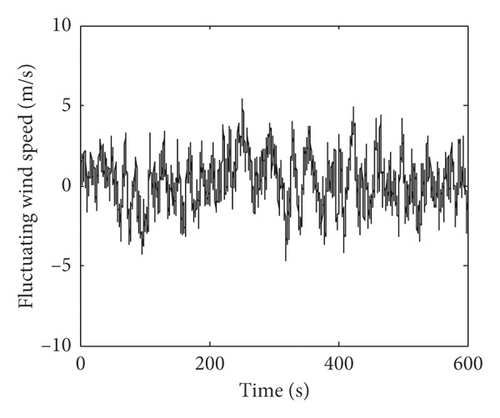
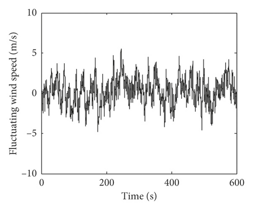
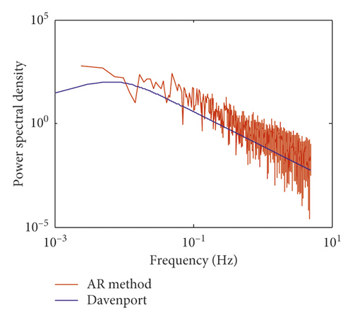
The fluctuating wind speed is numerically simulated based on the autoregressive model method. The power spectral density is Davenport spectral. The vertical wind profile is taken as the power profile with an exponent of a = 0.22 and a reference height of z_G = 10 m according to the Chinese National Load Code [32]. The mean wind speed at the reference height is 10 m/s. Figure 1 shows the simulated fluctuating wind speed on the fifth and tenth floors. Figure 2 shows the comparison of the power spectral density between the simulated fluctuating wind speed and the Davenport spectral on the fifth and tenth floors. Figure 2 shows that the simulated power spectral density matches very well with the Davenport spectral. The wind load acting on the building structure is calculated according to [22]. The air density is assumed to be ρ = 1.29 kg/m³. The drag coefficient is set to 1.3, and the orthogonal exposed wind area of each floor is set to 50 m².

Details are in the caption following the image — **Figure 1 (a)**
Open in figure viewer PowerPoint

Simulated fluctuating wind speed on the (a) fifth floor and (b) tenth floor.

3.1. Joint State/Parameter/Wind Load Estimation Based on Incomplete Measurements

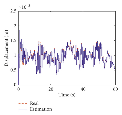
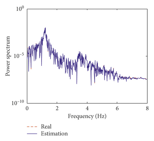
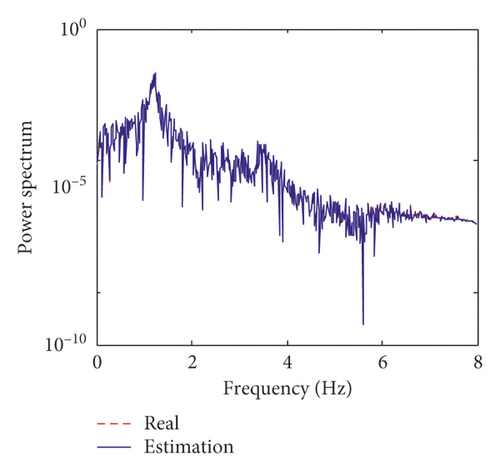
In this section, the interstory displacement and acceleration taken as the “measurements” are calculated based on the Newmark-β method and superimposed with 2% root mean square (RMS) white noise. Only seven sets of measurements including seven accelerations and seven interstory displacements are used for the estimation. The locations of the measurements are listed in Table 1. The unknown structural parameters are structural stiffness coefficients on each floor and the two Rayleigh damping coefficients. The initial value of the augmented state vector is $Z_{1| 0} = [\begin{matrix} 0_{120 \times} & 1.3 k & 1.3 α & 1.3 β \end{matrix}]$ , where k = [k₁, k₂, …, k₉, k₁₀]. The initial error covariance matrix of the augmented state vector is $P_{1 |0}^{Z} = diag ([\begin{matrix} {(1,11, \dots,)}_{120 \times} & {(10^{23}, 10^{23}, \dots, 10^{23})}_{110 \times} \end{matrix} {, 10}^{7} {, 10}^{2}])$ . The covariance matrix of process noise is Q = 10⁻², and the covariance matrix of measurement noise is R = 10⁻¹. Figure 3 shows the comparison of the estimated structural displacement responses with exact values on the fifth and tenth floors for time and frequency domains. Figure 4 shows the comparison of the estimated structural velocity responses with exact values on the fifth and tenth floors for time and frequency domains. The estimated curves coincide with the exact curves. This indicates that the proposed method is capable of identifying structural responses. Furthermore, two obvious peaks at 1.185 Hz and 3.527 Hz can be obtained in Figures 3 and 4. The two peaks correspond to the first two translational natural frequency of the building.

Table 1. Number of measurements and corresponding locations.

Number of measurements	Location (floor)
7	2, 3, 4, 5, 7, 9, 10

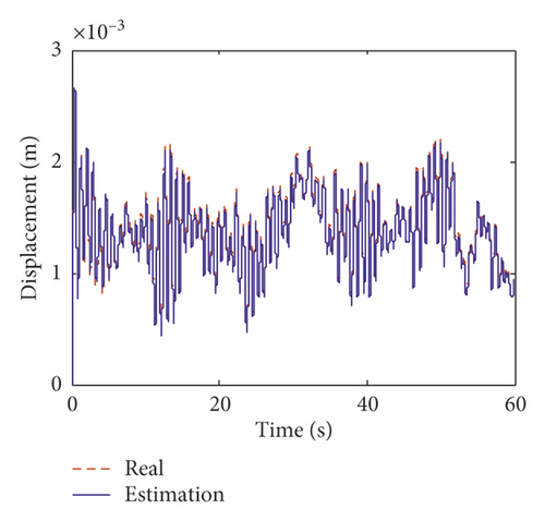
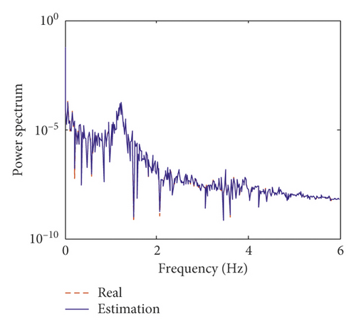
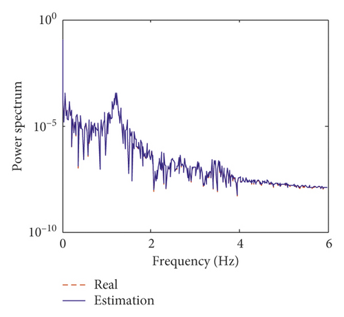
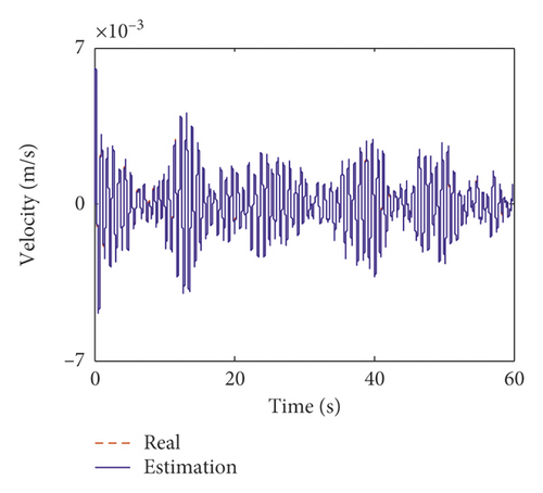
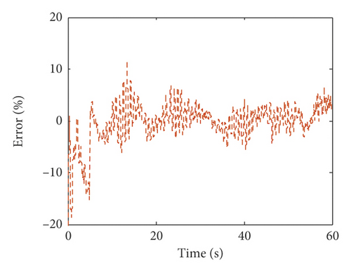
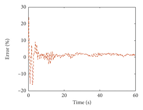
Moreover, based on the proposed method, the unknown wind load is identified using incomplete measurements. The identified wind load and the relative errors between the identified wind load and the exact one in percentage on the fifth and tenth floors of the numerical model are plotted in Figure 5. Figure 5 shows that the iteration process cannot converge immediately, but after approximately 8 s, the relative errors are well converged to less than 5%. Table 2 shows the mean errors and the RMS errors between the identified wind loads and the exact ones on each floor. From Table 2, the maximum mean errors and RMS errors of the identified wind loads are 4.12% and 4.56%, respectively. This means that the identified wind loads match the exact ones very well after iterative convergence.

Table 2. Mean errors and RMS errors for wind load estimation.

Floor number	Mean error (%)	RMS error (%)	Floor number	Mean error (%)	RMS error (%)
1	0.22	4.11	6	4.09	4.56
2	3.88	4.17	7	3.68	3.82
3	4.12	4.31	8	3.89	4.21
4	3.01	3.49	9	3.21	3.30
5	0.38	3.87	10	1.16	2.92

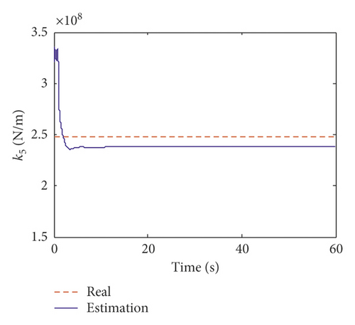
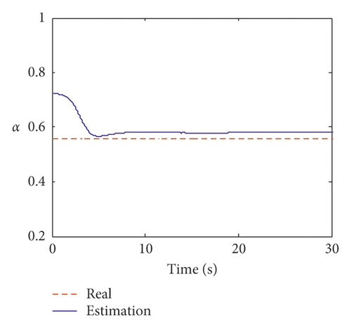
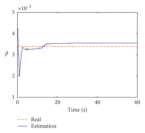
Figure 6 shows the estimated results of the fifth and tenth structural stiffness coefficients. It indicates that the stiffness coefficients can converge to the real value within 2 s. The estimation results of Rayleigh damping coefficients α and β are plotted in Figure 7. Compared to the stiffness coefficient, the damping coefficient converges slightly slower and can converge to a real value within approximately 5 s. Table 3 lists the estimated values and errors of the structural parameters. The maximum error for the stiffness coefficient is 4.30%. The estimated errors for the damping coefficients α and β are 4.25% and 4.24%, respectively. This indicates that the proposed method is capable of identifying the structural parameters with incomplete measurements.

Table 3. Estimation values and errors of structural parameters.

Structural parameter	Estimated value	Error (%)	Structural parameter	Estimated value	Error (%)
k₁	2.55 × 10⁸	3.97	k₇	2.55 × 10⁸	4.08
k₂	2.37 × 10⁸	3.44	k₈	2.55 × 10⁸	4.19
k₃	2.35 × 10⁹	4.15	k₉	2.53 × 10⁸	3.37
k₄	2.54 × 10⁸	3.84	k₁₀	2.34 × 10⁸	4.30
k₅	2.35 × 10⁸	3.96	α	5.81 × 10⁻¹	4.25
k₆	2.35 × 10⁸	3.99	β	3.58 × 10⁻³	4.24

3.1.1. Effect of Sampling Duration

To investigate the stability of the proposed method, the effect of the sampling duration on wind load and structural parameter estimation is discussed. The number and location of measurements are the same as in Table 1. The total duration of the measurements is set to 1 s, 10 s, 30 s, and 60 s. Table 4 shows the RMS errors of the estimated wind load on each floor under different sampling durations. The estimated results of the structural parameters are given in Table 5. From Table 4, the maximum RMS errors of wind load under 1 s, 10 s, 30 s, and 60 s are 14.23%, 7.68%, 4.58%, and 4.55%, respectively. From Table 5, the maximum errors of the structural parameters under 1 s, 10 s, 30 s, and 60 s are 32.78%, 6.99%, 4.66%, and 4.25%, respectively. This indicates that the estimation errors decrease as the time duration increases. Table 5 shows that the estimation errors of the wind load and structural parameters are all less than 5% when the sampling duration reaches 30 s. Furthermore, comparing the estimated results between 30 s and 60 s shows that the estimation accuracy increases slightly. Therefore, considering the computational costs, the sampling duration of 30 s is adequate for this numerical simulation.

Table 4. RMS errors of the estimated wind load under different sampling durations.

Floor number	RMS error (%)
Floor number	Duration: 1 s	Duration: 10 s	Duration: 30 s	Duration: 60 s
1	7.77	6.33	4.52	4.11
2	5.86	5.68	4.45	4.17
3	5.83	5.20	4.45	4.31
4	6.65	5.92	3.97	3.49
5	14.23	7.68	4.03	3.87
6	7.46	5.15	4.58	4.55
7	7.30	5.74	3.92	3.82
8	6.23	5.41	4.35	4.21
9	7.55	6.54	3.34	3.30
10	11.94	6.20	3.81	2.92

Table 5. Structural parameter estimation results under different sampling durations.

Structural parameter	Duration: 1 s		Duration: 10 s		Duration: 30 s		Duration: 60 s
Structural parameter	Estimated value	Error (%)	Estimated value	Error (%)	Estimated value	Error (%)	Estimated value	Error (%)
k₁	2.59 × 10⁸	5.86	2.57 × 10⁸	4.98	2.55 × 10⁸	4.12	2.55 × 10⁸	3.97
k₂	2.33 × 10⁸	4.89	2.36 × 10⁸	3.55	2.37 × 10⁸	3.45	2.37 × 10⁸	3.44
k₃	2.36 × 10⁸	3.76	2.37 × 10⁸	3.39	2.35 × 10⁸	4.20	2.35 × 10⁸	4.15
k₄	2.56 × 10⁸	4.55	2.55 × 10⁸	4.14	2.55 × 10⁸	4.15	2.54 × 10⁸	3.84
k₅	2.59 × 10⁸	5.61	2.57 × 10⁸	4.84	2.35 × 10⁸	4.01	2.35 × 10⁸	3.96
k₆	2.26 × 10⁸	7.62	2.28 × 10⁸	6.99	2.35 × 10⁸	4.02	2.35 × 10⁸	3.99
k₇	2.56 × 10⁸	4.41	2.55 × 10⁸	4.08	2.55 × 10⁸	4.09	2.55 × 10⁸	4.08
k₈	2.56 × 10⁸	4.35	2.55 × 10⁸	4.21	2.55 × 10⁸	4.21	2.55 × 10⁸	4.19
k₉	2.55 × 10⁸	4.06	2.53 × 10⁸	3.36	2.53 × 10⁸	3.40	2.53 × 10⁸	3.37
k₁₀	2.28 × 10⁸	6.97	2.29 × 10⁸	6.53	2.34 × 10⁸	4.52	2.34 × 10⁸	4.3
α	0.740	32.78	0.575	3.28	0.581	4.66	0.581	4.25
β	0.00440	29.33	0.00325	4.37	0.00348	3.49	0.00348	2.24

3.1.2. Effect of the Number of Measurements

This section discusses the influence of the number of measurements for joint state/parameter/wind load estimation. The considered set of measurements is four to nine, and each set of measurements includes interstory displacement and acceleration responses. Table 6 shows the number of measurements and the corresponding locations.

Table 6. Number of measurements and corresponding locations.

Number of measurements	Location (floor)
9	1, 2, 3, 5, 6, 7, 8, 9, 10
8	1, 3, 4, 5, 6, 8, 9, 10
7	2, 3, 4, 5, 7, 9, 10
6	1, 2, 4, 6, 8, 10
5	2, 4, 6, 8, 10
4	1, 4, 6, 9

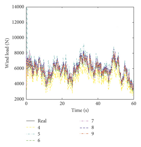
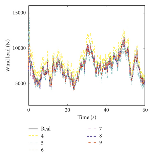
The time histories of the estimated wind loads on the fifth and tenth floors under different numbers of measurements are plotted in Figure 8. Figure 8 shows that the variation trends of the identified wind loads are identical to the exact ones. However, there is an obvious error between the estimated value and the exact one when the number of measurements is less than six. The RMS errors of the identified wind load on each floor under different numbers of measurements are listed in Table 7. Table 7 shows that as the number of measurements increases, the RMS error of the estimated wind load decreases. The maximum error under six, five, and four sets of measurements is 5.33%, 7.08%, and 10.78%, respectively. This indicates that the estimation error increases significantly when the number of measurements is less than six.

Table 7. RMS errors of wind load for different numbers of measurements.

Floor number	Nine measurements	Eight measurements	Seven measurements	Six measurements	Five measurements	Four measurements
1	2.43	3.47	4.11	4.77	6.27	9.29
2	2.4	3.06	4.17	4.71	5.14	10.6
3	2.06	3.24	4.31	4.7	6.38	8.12
4	2.34	3.01	3.49	4.38	6.09	10.78
5	2.43	3.15	3.87	4.51	7.08	9.2
6	2.98	3.42	4.56	5.33	5.59	8.23
7	2.49	3.3	3.82	4.58	6.03	10.06
8	2.24	3.45	4.21	4.77	5.77	9.2
9	0.81	2.31	3.3	4.95	6.30	8.05
10	1.1	2.42	2.92	3.48	5.94	9.25

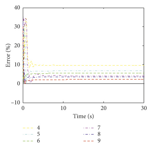
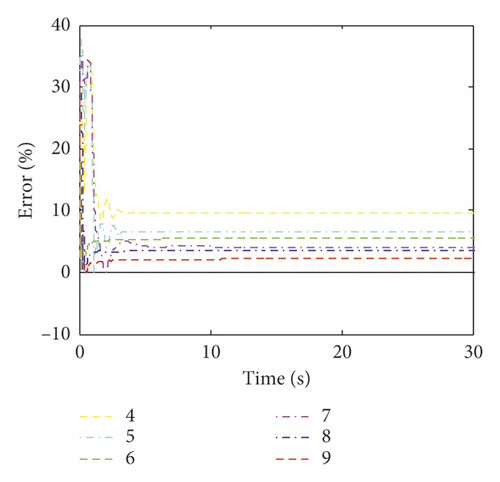
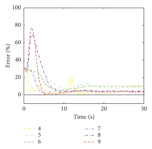
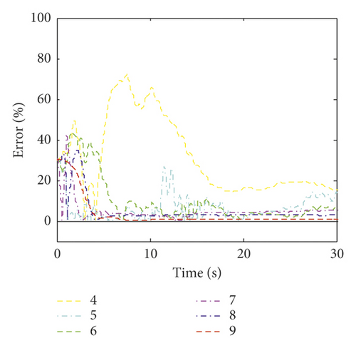
The time histories of the estimated errors of the fifth and tenth structural stiffness coefficients for different numbers of measurements are shown in Figure 9. Figure 9 shows that at the beginning of the iteration are some fluctuations. However, after approximately 2 s, the iteration converges to the true value. Figure 10 plots the estimated errors of damping coefficients α and β. Figure 10 shows that both α and β have a large fluctuation at the beginning of the iteration, and they converge to the true value after approximately 10 s under more than seven measurements. However, the estimation results fluctuate around the true value when the number of measurements is less than seven. This indicates that damping coefficients are sensitive to the number of measurements and fluctuate around the true value if the number of measurements is insufficient. Table 8 gives the estimation results of the structural parameters with the number of measurements (i.e., from 4 to 9). The maximum errors of the estimated parameters under four to nine measurements are 13.01%, 11.76%, 9.83%, 4.30%, 3.71%, and 3.63%, respectively. It indicates that as the number of measurements increases, the estimation accuracy of the structural parameters increases. The maximum errors of the structural stiffness coefficient and the damping coefficients α and β under six sets of measurements are 5.98%, 9.83%, and 5.33%, respectively. However, the estimation errors of each structural parameter are less than 5% under seven sets of measurements. The results indicate that, for this particular example, at least seven sets of measurements should be used.

Table 8. Estimation of structural parameters under different numbers of measurements.

Structural parameter	Nine measurements		Eight measurements		Seven measurements		Six measurements		Five measurements		Four measurements
Structural parameter	Value (×10⁸)	Error (%)	Value (×10⁸)	Error (%)	Value (×10⁸)	Error (%)	Value (×10⁸)	Error (%)	Value (×10⁸)	Error (%)	Value (×10⁸)	Error (%)
k₁	2.52	2.81	2.37	3.38	2.55	3.97	2.35	4.12	2.61	6.52	2.68	9.51
k₂	2.39	2.56	2.52	2.88	2.37	3.44	2.55	4.02	2.60	6.28	2.68	9.48
k₃	2.40	2.03	2.37	3.12	2.35	4.15	2.34	4.31	2.58	5.45	2.21	9.62
k₄	2.40	1.97	2.53	3.24	2.54	3.84	2.30	5.98	2.61	6.44	2.22	9.26
k₅	2.51	2.35	2.53	3.44	2.35	3.96	2.59	5.65	2.28	6.74	2.69	9.64
k₆	2.51	2.26	2.38	2.76	2.35	3.99	2.57	5.07	2.29	6.39	2.70	10.08
k₇	2.38	2.86	2.37	3.42	2.55	4.08	2.57	4.94	2.30	6.27	2.68	9.25
k₈	2.39	2.28	2.52	2.98	2.55	4.19	2.32	5.43	2.62	6.74	2.71	10.46
k₉	2.49	1.50	2.51	2.49	2.53	3.37	2.55	4.25	2.29	6.73	2.67	9.18
k₁₀	2.50	2.12	2.53	3.40	2.34	4.30	2.58	5.43	2.29	6.62	2.69	9.61
Α × 10⁸	0.577	3.63	0.581	3.71	0.581	4.25	0.612	9.83	0.592	6.27	0.606	8.71
β × 10⁸	0.00342	0.76	0.0035	2.8	0.00348	2.24	0.00358	5.33	0.0038	11.76	0.00384	13.01

4. Validation with Wind Tunnel Tests

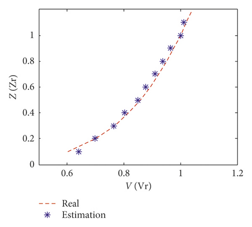
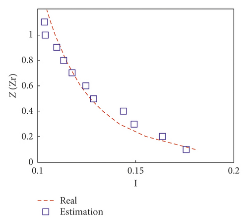
In order to verify the effectiveness of the proposed method in practical engineering application, a tall building with 58 floors is considered as an example in this study. The size of the building is 234 m (height) × 39 m (width) × 39 m (length). The synchronous multipressure scanning system wind tunnel test for simultaneous estimation of state, unknown structural parameters, and wind load was conducted in wind environment wind tunnel laboratory at Harbin Institute of Technology (Shenzhen), China. According to Chinese National Load Code (GB 50009-2012) [32], the site around the test building is taken as terrain C. The wind profile is regarded as power law with an exponent of 0.22. The length scale of this wind tunnel test is 1 : 300. Figure 11 shows the simulated profiles of mean wind speed and turbulence intensity.

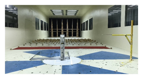
The model has the same length scale with that of wind field simulation, i.e., 1 : 300. The size of the model is 780 mm (height) × 130 mm (width) × 130 mm (length), as shown in Figure 12. In this wind tunnel test, wind direction was defined as an angle θ_d from 0° to 360° with increments of 15°, as shown in Figure 13. The total number of the pressure taps installed on the building was 441 with 98 on each side surface and 49 on top surface. The pressure data were collected using an microelectronic pressure scanner system made by PSI. The data sampling frequency was 330 Hz, and the sampling length was 120 s. The wind speed at the top of the model with a 10-year return period is 39.6 m/s based on Chinese National Load Code [32].

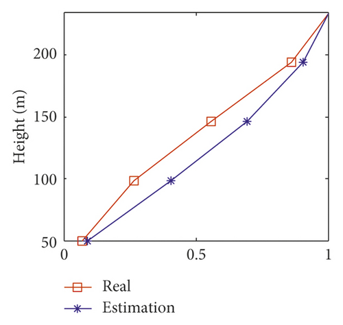
4.1. Equivalent Model of the Tall Building

For building structures with large degrees-of-freedom, it is complicated or even impossible to estimate the wind load and structural parameters strictly according to the prototype structure. Generally, a simplified equivalent model with less degrees-of-freedom is needed in practical analysis. The equivalent model requires that the vibration responses of the two systems are same. This means that the work-energy between the prototype structure and the equivalent structure is equal. Based on the method proposed in [33], the equivalent mass and equivalent stiffness can be obtained as follows:

\begin{matrix} M_{e} = \frac{E \{\int_{0}^{H_{i}} m (z) {\dot{x}}^{2} (z, t) d z\}}{E \{{\dot{x}}_{0}^{2} + {\dot{x}}_{H_{i}}^{2}\}}, \\ K_{e} = \frac{E \{\int_{0}^{H_{i}} k (z) x^{2} (z, t) d z\}}{E \{x_{0}^{2} + x_{H_{i}}^{2}\}}, \end{matrix}

(53)

in which m(z) is the mass distribution of the prototype structure, k(z) is the stiffness distribution of the prototype structure, x(z, t) is the displacement of the prototype structure, M_e is the equivalent mass, and K_e is the equivalent stiffness.

Based on the mode decomposition method, the displacement can be represented as follows:

\begin{matrix} x (z, t) = \sum_{j} Y_{j} (t) φ_{j} (z), \end{matrix}

(54)

where Y_j(t) is the j-th modal displacement and φ_j(z) is the j-th mode shape vector. For tall building structures, the first mode is taken as the main mode of vibration. Then, the equivalent mass and equivalent stiffness can be calculated as follows:

\begin{matrix} M_{e} = \frac{\int_{0}^{H_{i}} m (z) φ_{i}^{2} (z) d z}{φ_{1}^{2} (0) + φ_{1}^{2} (H_{i})}, \end{matrix}

(55)

\begin{matrix} K_{e} = \frac{\int_{0}^{H_{i}} k (z) φ_{i}^{2} (z) d z}{φ_{1}^{2} (0) + φ_{1}^{2} (H_{i})} . \end{matrix}

(56)

Table 9 lists the energy contribution κ of the first five modal acceleration responses, modal velocity responses, and modal displacement responses, which are calculated according to the following equation:

\begin{matrix} κ = \frac{\sum_{i = 1}^{i = m} σ_{i}}{\sum_{i = 1}^{i = n} σ_{i}}, 1 \leq m \leq n, \end{matrix}

(57)

where σ_i is the mean squared value of the responses calculated based on proper orthogonal decomposition [34]. It can be seen that energy contribution of the first five modes is over 99%. Therefore, the simplified equivalent model is chosen as a shear building structure with five degrees-of-freedom. Assume that the simplified model quality is concentrated on the 12th, 24th, 36th, 48th, and 58th floors corresponding to the height of 50 m, 98 m, 146 m, 194 m, and 234 m, respectively. The equivalent mass coefficients and stiffness coefficients are calculated based on Equations (55) and (56), respectively, which are shown in Table 10. Table 11 gives the first five natural frequencies of the prototype structure and the equivalent model. It can be found that the relative errors of the first three natural frequencies are under 5%. Figure 14 shows the comparison of the first two mode shapes between the prototype structure and the equivalent structure. It can be found that the mode shapes of the equivalent structure are consistent with that of the prototype structure. The damping of this structure is considered as Rayleigh damping with damping ratio corresponding to the first two modes of vibration being 5%.

Table 9. Energy contribution ratio of the first five modal responses.

Number of modes	1	2	3	4	5
Displacement	99.458	99.963	99.994	99.999	99.999
Velocity	98.068	99.673	99.898	99.963	99.989
Acceleration	85.276	94.096	96.825	98.396	99.369

Table 10. Equivalent mass and stiffness of the equivalent model.

Floor number	1	2	3	4	5
M_e	3.62 × 10⁷	2.38 × 10⁷	2.30 × 10⁷	2.11 × 10⁷	1.16 × 10⁷
K_e	9.53 × 10⁸	2.52 × 10⁸	2.30 × 10⁸	2.04 × 10⁸	1.74 × 10⁸

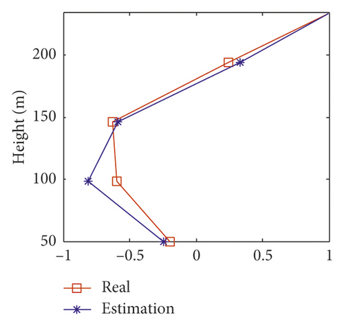
Table 11. Comparison of the first five natural frequencies between the prototype model and the equivalent model.

Modal order	1	2	3	4	5
Real value	0.19	0.49	0.77	1.07	1.35
Simplified model	0.19	0.51	0.76	0.90	1.00
Error (%)	2.48	4.16	2.34	15.50	26.10

4.2. Wind Load and Structural Parameters Estimation

The wind-induced responses of the tall building cannot be measured directly from the pressure measurement on a rigid model in the wind tunnel test. Hence, wind-induced responses including displacement, velocity, and acceleration responses are calculated based on the wind tunnel test results and the structural dynamic properties of the prototype building structure using the Newmark-β method. In order to validate the feasibility of the proposed method, only three sets of measurements including structural interstory displacement responses and acceleration responses on the 12th, 36th, and 58th floors are taken as the “measurements.” The unknown parameters are five stiffness coefficients and two Rayleigh damping coefficients of the equivalent model. The unknown excitations are equivalent wind load on the equivalent model. The initial value of the state vector is $Z_{1| 0} = [\begin{matrix} 0_{110 \times} & 1.3 k & 1.3 α & 1.3 β \end{matrix}]$ . The initial error covariance matrix is $P_{1| 0}^{Z} = diag (\begin{matrix} {[1,11, \dots,]}_{110 \times} & {(10^{25} {, 10}^{25}, \dots, 10^{25})}_{110 \times} & 10^{3} & 10^{1} \end{matrix})$ . The covariance matrices of process noise and measurement noise are 10⁻² and 10⁻¹, respectively.

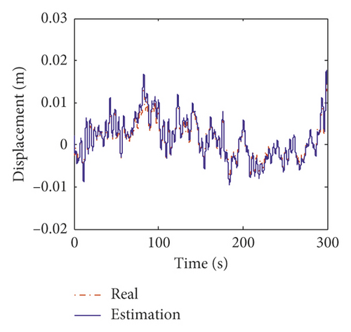
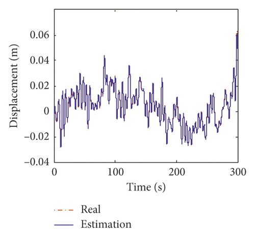
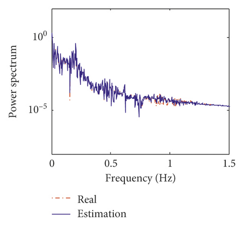
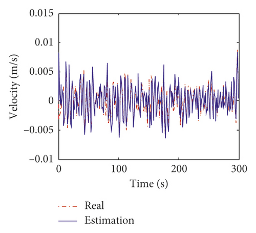
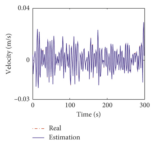
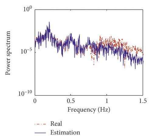
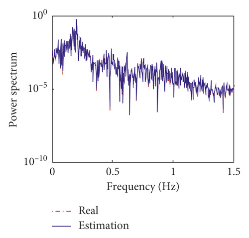
Figures 15 and 16 show the estimation results of structural displacement responses and velocity responses on the 24th and 58th floors, respectively. It can be found that the time histories of the estimated responses match very well with the exact responses. Meanwhile, the power spectrum of the estimated responses is found to agree well with those of the exact responses except slight differences in high frequency components (>0.8 Hz) of the responses on the 24th floor. This is mainly because (1) there is no measurement information on the 24th floor, and the estimation results on the 24th floor is obtained from modal transformation and (2) the errors of the modal information between the equivalent model and prototype model are large in higher modes (i.e., the fourth and fifth modes).

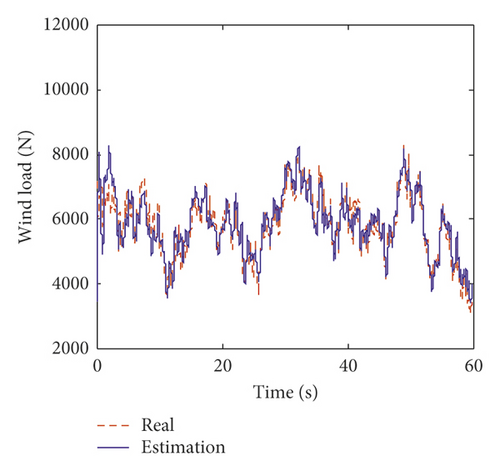
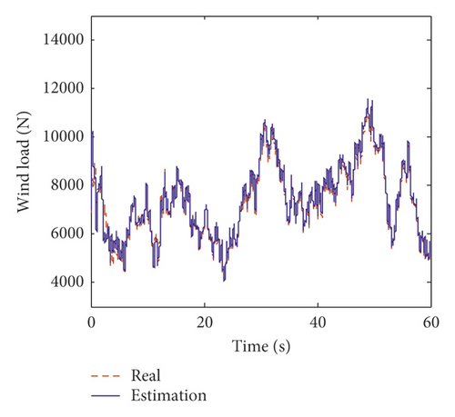
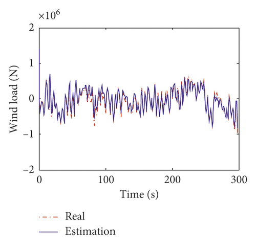
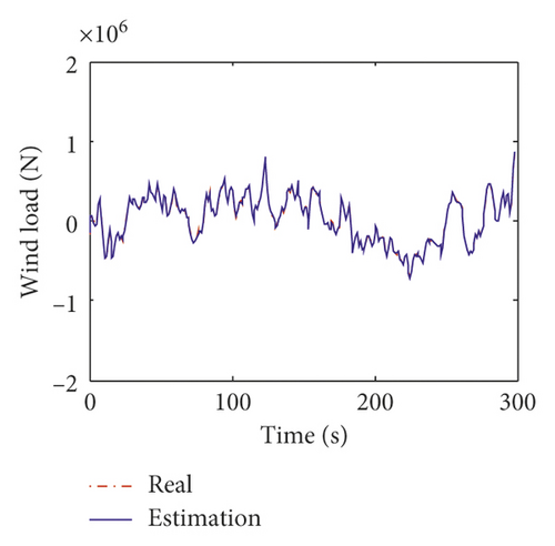
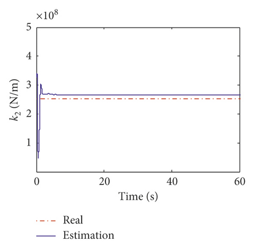
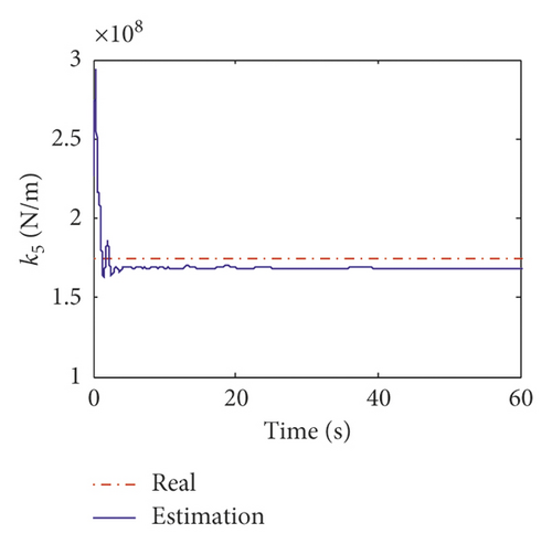
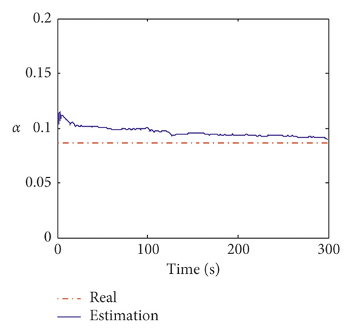
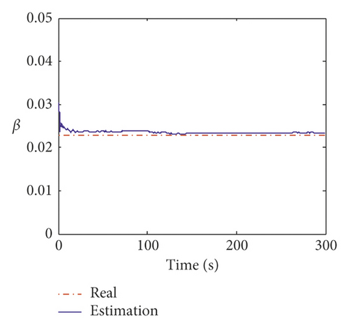
Displayed in Figure 17 is the comparison of the time histories of the equivalent wind load between the exact values and estimated values on the 24th floor and 58th floor. It can be observed that the estimated curves agree very well with the exact ones. The estimation errors of the equivalent wind load are listed in Table 12. From Table 12, the maximum mean error and RMS error of the identified wind load are 4.95% and 5.89%. Figure 18 shows the estimation results of the equivalent stiffness coefficients. It indicates that the stiffness coefficients can converge to the real value within 5 s. The estimation results of damping coefficients are shown in Figure 19, and it can be found that the damping coefficients can converge to the real value within about 10 s. The estimated values and errors of structural parameters are given in Table 13. The errors of the stiffness coefficient are less than 5% except that on the 12th floor. The errors of the damping coefficient α and β are 3.8% and 2.11%, respectively. The comparison results indicate that the inverse method presented in this study is applicable to the practical engineering.

Table 12. Mean errors and RMS errors for wind load estimation.

Floor number	12	24	36	48	58
Mean value	4.95	4.59	−4.87	4.29	4.93
RMS	1.63	3.85	5.27	5.55	5.89

Table 13. Estimation values and errors of structural parameters.

Structural parameter	True value	Estimated value	Errors (%)
k₁	9.53 × 10⁸	9.02 × 10⁸	5.40
k₂	2.52 × 10⁸	2.62 × 10⁸	4.25
k₃	2.30 × 10⁸	2.20 × 10⁸	4.41
k₄	2.04 × 10⁸	1.94 × 10⁸	4.81
k₅	1.74 × 10⁸	1.66 × 10⁸	4.52
α	0.086	0.0898	3.80
β	0.023	0.0234	2.11

5. Conclusion

In this paper, a time domain joint state/parameter/wind load estimation method from incomplete measurements is proposed based on modal extended unbiased minimum variance estimation. The recursive procedure includes four parts: time update, modal wind load estimation, measurement update, and coordinate transformation. The measurement responses include the interstory displacement and acceleration responses on partial floors. The estimation quality of the proposed method is numerically validated by simultaneously identifying the structural state, parameters, and wind load of a ten-story shear building structure from incomplete measurements. The effects of crucial factors, including sampling duration and the number of measurements on the convergence and accuracy of the proposed method, are discussed. Moreover, a synchronous multipressure scanning system wind tunnel test on a 234 m tall building structure is used to demonstrate the proposed approach for real structure. A simplified equivalent model with five degrees-of-freedom is derived for experimental validation. Results indicate that the proposed method shows much potential as an alternative way for simultaneously identify the unknown structural parameters, wind load, and wind-induced responses from incomplete measurements.

Conflicts of Interest

The authors declare that there are no conflicts of interest regarding the publication of this article.

Acknowledgments

This work was supported by the National Nature Science Foundation of China (Grant no. 51608153) and Shenzhen Knowledge Innovation Programme (Grant nos. JCYJ20170413105418298, JCYJ20180306171737796, and JCYJ20170811153857358).

Open Research

Data Availability

The data used to support the findings of this study are available from the corresponding author upon request.

References

1 He Y. C. and Li Q., Dynamic responses of a 492 m-high tall building with active tuned mass damping system during a typhoon, Structural Control and Health Monitoring. (2014) 21, 705–720, https://doi.org/10.1002/stc.1596, 2-s2.0-84897574474.
10.1002/stc.1596
Web of Science® Google Scholar
2 Li Q. S., Zhi L.-H., Tuan A. Y., Kao C.-S., Su S.-C., and Wu C.-F., Dynamic behavior of Taipei 101 tower: field measurement and numerical analysis, Journal of Structural Engineering. (2011) 137, no. 1, 143–155, https://doi.org/10.1061/(asce)st.1943-541x.0000264, 2-s2.0-78650408028.
10.1061/(ASCE)ST.1943-541X.0000264
Web of Science® Google Scholar
3 Mendis P., Ngo T., Haritos N., Hira A., Samali B., and Cheung J., Wind loading on tall buildings, Electronic Journal of Structural Engineering. (2007) 7, 41–54.
10.56748/ejse.641
Google Scholar
4 Simiu E. and Scanlan R. H., Wind Effects on Structures: Fundamentals and Applications to Design, 1996, John Wiley, Hoboken, NJ, USA.
Google Scholar
5 Zhou Y., Kijewski T., and Kareem A., Along-wind load effects on tall buildings: comparative study of major international codes and standards, journal of Structural Engineering. (2002) 128, no. 6, 788–796, https://doi.org/10.1061/(asce)0733-9445(2002)128:6(788), 2-s2.0-0344758130.
10.1061/(ASCE)0733-9445(2002)128:6(788)
Web of Science® Google Scholar
6 Huang S., Li Q. S., and Xu S., Numerical evaluation of wind effects on a tall steel building by CFD, Steel Construction. (2008) 63, no. 5, 612–627, https://doi.org/10.1016/j.jcsr.2006.06.033, 2-s2.0-33751350597.
10.1016/j.jcsr.2006.06.033
CAS Google Scholar
7 Li Q. S., Fu J. Y., Xiao Y. Q. et al., Wind tunnel and full-scale study of wind effects on China’s tallest building, Engineering Structures. (2006) 28, no. 12, 1745–1758, https://doi.org/10.1016/j.engstruct.2006.02.017, 2-s2.0-33746627738.
10.1016/j.engstruct.2006.02.017
PubMed Web of Science® Google Scholar
8 Uhl T., The inverse identification problem and its technical application, Archive of Applied Mechanics. (2007) 77, no. 5, 325–337, https://doi.org/10.1007/s00419-006-0086-9, 2-s2.0-34248351921.
10.1007/s00419-006-0086-9
Web of Science® Google Scholar
9 Desanghere G., Indirect identification of excitation forces by modal coordinate transformation, Proceedings of the 3rd International Modal Analysis Conference, January 1985, Orlando, FL, USA.
Google Scholar
10 Kim Y.-R. and Kim K.-J., Indirect input identification by modal filter technique, Mechanical Systems and Signal Processing. (1999) 13, no. 6, 893–910, https://doi.org/10.1006/mssp.1999.1240, 2-s2.0-0033311905.
10.1006/mssp.1999.1240
Web of Science® Google Scholar
11 Law S. S., Bu J. Q., and Zhu X. Q., Time-varying wind load identification from structural responses, Engineering Structures. (2005) 27, no. 10, 1586–1598, https://doi.org/10.1016/j.engstruct.2005.05.007, 2-s2.0-21044448821.
10.1016/j.engstruct.2005.05.007
Web of Science® Google Scholar
12 Lu Z. R. and Law S. S., Force identification based on sensitivity in time domain, Journal of Engineering Mechanics. (2006) 132, no. 10, 1050–1056, https://doi.org/10.1061/(asce)0733-9399(2006)132:10(1050), 2-s2.0-33748766361.
10.1061/(ASCE)0733-9399(2006)132:10(1050)
Web of Science® Google Scholar
13 Liu Y. and Shepard W. S., Dynamic force identification based on enhanced least squares and total least-squares schemes in the frequency domain, Journal of Sound & Vibration. (2005) 282, no. 1-2, 37–60, https://doi.org/10.1016/j.jsv.2004.02.041, 2-s2.0-17844379998.
10.1016/j.jsv.2004.02.041
Web of Science® Google Scholar
14 Liu J.-J., Ma C.-K., Kung I.-C., and Lin D.-C., Input force estimation of a cantilever plate by using a system identification technique, Computer Methods in Applied Mechanics and Engineering. (2000) 190, no. 11-12, 1309–1322, https://doi.org/10.1016/s0045-7825(99)00465-x, 2-s2.0-0034501580.
10.1016/S0045-7825(99)00465-X
Web of Science® Google Scholar
15 Ma C.-K., Tuan P.-C., Lin D.-C., and Liu C.-S., A study of an inverse method for the estimation of impulsive loads, International Journal of Systems Science. (1998) 29, no. 6, 663–672, https://doi.org/10.1080/00207729808929559, 2-s2.0-0032098904.
10.1080/00207729808929559
Web of Science® Google Scholar
16 Hwang J.-s., Kareem A., and Kim W.-j., Estimation of modal loads using structural response, Journal of Sound and Vibration. (2009) 326, no. 3–5, 522–539, https://doi.org/10.1016/j.jsv.2009.05.003, 2-s2.0-67849115988.
10.1016/j.jsv.2009.05.003
Web of Science® Google Scholar
17 Hwang J.-S., Kareem A., and Kim H., Wind load identification using wind tunnel test data by inverse analysis, Journal of Wind Engineering and Industrial Aerodynamics. (2011) 99, no. 1, 18–26, https://doi.org/10.1016/j.jweia.2010.10.004, 2-s2.0-78650265711.
10.1016/j.jweia.2010.10.004
Web of Science® Google Scholar
18 Zhi L. H., Fang M. X., and Li Q. S., Estimation of wind loads on a tall building by an inverse method, Structural Control & Health Monitoring. (2017) 24, no. 4, https://doi.org/10.1002/stc.1908, 2-s2.0-84979080281.
10.1002/stc.1908
Web of Science® Google Scholar
19 Zhi L., Li Q. S., Fang M., and Yi J., Identification of wind loads on super tall buildings using kalman filtering–based inverse method, Journal of Structural Engineering. (2016) 143, no. 4, 06016004, https://doi.org/10.1061/(asce)st.1943-541x.0001691, 2-s2.0-85015927250.
10.1061/(ASCE)ST.1943-541X.0001691
Web of Science® Google Scholar
20 Gillijns S. and De Moor B., Unbiased minimum-variance input and state estimation for linear discrete-time systems with direct feedthrough, Automatica. (2007) 43, no. 5, 934–937, https://doi.org/10.1016/j.automatica.2006.11.016, 2-s2.0-34047159828.
10.1016/j.automatica.2006.11.016
Web of Science® Google Scholar
21 Lourens E., Papadimitriou C., Gillijns S., Reynders E., De Roeck G., and Lombaert G., Joint input-response estimation for structural systems based on reduced-order models and vibration data from a limited number of sensors, Mechanical Systems and Signal Processing. (2012) 29, 310–327, https://doi.org/10.1016/j.ymssp.2012.01.011, 2-s2.0-84859433776.
10.1016/j.ymssp.2012.01.011
Web of Science® Google Scholar
22 Xue H., Lin K., Luo Y., and Liu H., Time-varying wind load identification based on minimum-variance unbiased estimation, Shock and Vibration. (2017) 2017, 1–15, https://doi.org/10.1155/2017/9301876, 2-s2.0-85042471783.
10.1155/2017/9301876
CAS Web of Science® Google Scholar
23 Wan Z., Wang T., Li L., and Xu Z., A novel coupled state/input/parameter identification method for linear structural systems, Shock and Vibration. (2018) 2018, 15, 7691721, https://doi.org/10.1155/2018/7691721, 2-s2.0-85043393988.
10.1155/2018/7691721
Web of Science® Google Scholar
24 Song W., Generalized minimum variance unbiased joint input-state estimation and its unscented scheme for dynamic systems with direct feedthrough, Mechanical Systems and Signal Processing. (2018) 99, 886–920, https://doi.org/10.1016/j.ymssp.2017.06.032, 2-s2.0-85026863968.
10.1016/j.ymssp.2017.06.032
Web of Science® Google Scholar
25 Kuhar E. J. and Stahle C. V., Dynamic transformation method for modal synthesis, AIAA Journal. (1973) 12, no. 5, 672–678, https://doi.org/10.2514/3.49318, 2-s2.0-0016059018.
10.2514/3.49318
Web of Science® Google Scholar
26 Liu L., Hua W., and Lei Y., Real-time simultaneous identification of structural systems and unknown inputs without collocated acceleration measurements based on MEKF-UI, Measurement. (2018) 122, 545–553, https://doi.org/10.1016/j.measurement.2017.07.001, 2-s2.0-85022089435.
10.1016/j.measurement.2017.07.001
Web of Science® Google Scholar
27 Alvin K. F., Efficient computation of eigenvector sensitivities for structural dynamics via conjugate gradients, Proceedings of the 16th International Modal Analysis Conference, February 1998, Santa Barabara, CA, USA, 652–659.
Google Scholar
28 Wang B. P., Improved approximate methods for computing eigenvector derivatives in structural dynamics, AIAA Journal. (1991) 29, no. 6, 1018–1020, https://doi.org/10.2514/3.59945, 2-s2.0-0026170497.
10.2514/3.59945
PubMed Web of Science® Google Scholar
29 Jones N. P., Shi T., Hugh Ellis J., and Scanlan R. H., System-identification procedure for system and input parameters in ambient vibration surveys, Journal of Wind Engineering and Industrial Aerodynamics. (1995) 54-55, 91–99, https://doi.org/10.1016/0167-6105(94)00033-a, 2-s2.0-0029102634.
10.1016/0167-6105(94)00033-A
Web of Science® Google Scholar
30 Rao C. R., Linear Statistical Inference and its Applications, 1973, Wiley, Hoboken, NJ, USA.
10.1002/9780470316436
Google Scholar
31 Kitanidis P. K., Unbiased minimum-variance linear state estimation, Automatica. (1987) 23, no. 6, 775–778, https://doi.org/10.1016/0005-1098(87)90037-9, 2-s2.0-0023456666.
10.1016/0005-1098(87)90037-9
Web of Science® Google Scholar
32 Gerges B., Load Code for the Design of Building Structures, 2012, China Architecture & Building Press, Beijing, China.
Google Scholar
33 Xiangting Z., Study of random vinration of major engineering structure for equivalent-lumped system based on work-enrygu principle, Shock and Vibration. (1995) 2, 7–11, in Chinese.
Google Scholar
34 Han S. and Feeny B., Application of proper orthogonal decomposition to structural vibration analysis, Mechanical Systems and Signal Processing. (2003) 17, no. 5, 989–1001, https://doi.org/10.1006/mssp.2002.1570, 2-s2.0-0037803533.
10.1006/mssp.2002.1570
Web of Science® Google Scholar

Citing Literature

All articles

Wind Load and Structural Parameters Estimation from Incomplete Measurements

Abstract

1. Introduction

2. Modal Extended Minimum Variance Unbiased Estimation

2.1. System Model

2.2. Eigenvalue and Eigenvector Sensitivity

2.3. Modal Extended Minimum Variance Unbiased Estimation

2.3.1. Time Update

2.3.2. Modal Wind Load Estimation

2.3.3. Measurement Update

3. Numerical Simulation

3.1. Joint State/Parameter/Wind Load Estimation Based on Incomplete Measurements

3.1.1. Effect of Sampling Duration

3.1.2. Effect of the Number of Measurements

4. Validation with Wind Tunnel Tests

4.1. Equivalent Model of the Tall Building

4.2. Wind Load and Structural Parameters Estimation

5. Conclusion

Conflicts of Interest

Acknowledgments

Open Research

Data Availability

References

Citing Literature

Figures

References

Information

About Wiley Online Library

Help & Support

Opportunities

Connect with Wiley

Wind Load and Structural Parameters Estimation from Incomplete Measurements

Abstract

1. Introduction

2. Modal Extended Minimum Variance Unbiased Estimation

2.1. System Model

2.2. Eigenvalue and Eigenvector Sensitivity

2.3. Modal Extended Minimum Variance Unbiased Estimation

2.3.1. Time Update

2.3.2. Modal Wind Load Estimation

2.3.3. Measurement Update

3. Numerical Simulation

3.1. Joint State/Parameter/Wind Load Estimation Based on Incomplete Measurements

3.1.1. Effect of Sampling Duration

3.1.2. Effect of the Number of Measurements

4. Validation with Wind Tunnel Tests

4.1. Equivalent Model of the Tall Building

4.2. Wind Load and Structural Parameters Estimation

5. Conclusion

Conflicts of Interest

Acknowledgments

Open Research

Data Availability

References

Citing Literature

Figures

References

Related

Information