Volume 2019, Issue 1 3154845

Research Article

Open Access

Fusion Algorithm-Based Temperature Compensation Method for High-G MEMS Accelerometer

Qing Lu,

Qing Lu

School of Instrument and Electronics, North University of China, Taiyuan 030051, China nuc.edu.cn

Search for more papers by this author

Chong Shen,

Chong Shen

orcid.org/0000-0002-6046-6051

School of Instrument and Electronics, North University of China, Taiyuan 030051, China nuc.edu.cn

Science and Technology on Electronic Test & Measurement Laboratory, North University of China, Taiyuan 030051, China nuc.edu.cn

Search for more papers by this author

Huiliang Cao,

Corresponding Author

Huiliang Cao

[email protected]

orcid.org/0000-0001-9862-4329

School of Instrument and Electronics, North University of China, Taiyuan 030051, China nuc.edu.cn

Science and Technology on Electronic Test & Measurement Laboratory, North University of China, Taiyuan 030051, China nuc.edu.cn

Search for more papers by this author

Yunbo Shi,

Yunbo Shi

School of Instrument and Electronics, North University of China, Taiyuan 030051, China nuc.edu.cn

Science and Technology on Electronic Test & Measurement Laboratory, North University of China, Taiyuan 030051, China nuc.edu.cn

Search for more papers by this author

Jun Liu,

Corresponding Author

Jun Liu

[email protected]

orcid.org/0000-0003-2766-183X

School of Instrument and Electronics, North University of China, Taiyuan 030051, China nuc.edu.cn

Science and Technology on Electronic Test & Measurement Laboratory, North University of China, Taiyuan 030051, China nuc.edu.cn

Search for more papers by this author

Qing Lu,

Qing Lu

School of Instrument and Electronics, North University of China, Taiyuan 030051, China nuc.edu.cn

Search for more papers by this author

Chong Shen,

Chong Shen

orcid.org/0000-0002-6046-6051

School of Instrument and Electronics, North University of China, Taiyuan 030051, China nuc.edu.cn

Science and Technology on Electronic Test & Measurement Laboratory, North University of China, Taiyuan 030051, China nuc.edu.cn

Search for more papers by this author

Huiliang Cao,

Corresponding Author

Huiliang Cao

[email protected]

orcid.org/0000-0001-9862-4329

School of Instrument and Electronics, North University of China, Taiyuan 030051, China nuc.edu.cn

Science and Technology on Electronic Test & Measurement Laboratory, North University of China, Taiyuan 030051, China nuc.edu.cn

Search for more papers by this author

Yunbo Shi,

Yunbo Shi

School of Instrument and Electronics, North University of China, Taiyuan 030051, China nuc.edu.cn

Science and Technology on Electronic Test & Measurement Laboratory, North University of China, Taiyuan 030051, China nuc.edu.cn

Search for more papers by this author

Jun Liu,

Corresponding Author

Jun Liu

[email protected]

orcid.org/0000-0003-2766-183X

School of Instrument and Electronics, North University of China, Taiyuan 030051, China nuc.edu.cn

Science and Technology on Electronic Test & Measurement Laboratory, North University of China, Taiyuan 030051, China nuc.edu.cn

Search for more papers by this author

First published: 2019

https://doi.org/10.1155/2019/3154845

Citations: 9

Academic Editor: Chao Tao

Share a link

Email
Wechat
Bluesky

Abstract

In recent years, High-G MEMS accelerometers have been widely used in aviation, medicine, and other fields. So it is extremely important to improve the accuracy and performance of High-G MEMS accelerometers. For this purpose, we propose a fusion algorithm that combines EMD, wavelet thresholding, and temperature compensation to process measurement data from a High-G MEMS accelerometer. In the fusion algorithm, the original accelerometer signal is first decomposed by EMD to obtain the intrinsic mode function (IMF). Then, sample entropy (SE) is used to divide the IMF components into three segments. The noise segment is directly omitted, wavelet thresholding is performed on the mixing segment, and a GA-BP performs temperature compensation on the drift segment. Finally, signal reconstruction is implemented. Later, a comparative analysis is carried out on the results from four models: EMD, wavelet thresholding, EMD + wavelet thresholding, and EMD + wavelet thresholding + temperature compensation. The experimental data show that the acceleration random walk change from 1712.66 g/h/Hz^0.5 to 79.15 g/h/Hz^0.5 and the zero-deviation stability change from 49275 g/h to 774.7 g/h. This indicates that the fusion algorithm (EMD + wavelet thresholding + temperature compensation) not only effectively suppresses the noise of high-frequency components but also compensates for temperature drift in the accelerometer.

1. Introduction

MEMS accelerometers are fabricated using MEMS technology [1]. The High-G MEMS accelerometer is a general term for high-range accelerometers. It is a key component in the inertial testing and control of MEMS technology for fusion intrusion. The main application of the High-G MEMS accelerometer is the measurement and control of speed changes in high-speed motion carriers during start-up and operation [2, 3]. Thus, the High-G MEMS accelerometer is widely used in the aerospace field for the precise control of missiles and intelligent projectiles [4]. Therefore, research on this type of sensor and the associated MEMS system is extremely significant. Many High-G MEMS accelerometers are the most susceptible component of the input system and critically affect the accuracy of the system. The effects of the accelerometer itself and the signal hardware acquisition circuit result in the superposition of the acquired accelerometer signal and a large number of noise signals. Direct analysis of the output signal inevitably produces an error that requires corresponding denoising processing [5]. The traditional Fourier transform filter operates on the difference between the frequency distributions of the signal and the noise. Thus, an undesirable frequency component can be removed by selecting an appropriate filter in the frequency domain to achieve denoising [6]. However, a precondition for processing using Fourier transforms is that the signal satisfies the stationary assumption. It is often difficult to denoise nonstationary or transient signals using frequency domain filtering methods, because the Fourier transform is not applicable to the nonstationary signals that are encountered in practice [7]. In empirical mode decomposition, the data themself are used to adaptively decompose nonstationary signals, such that arbitrary nonlinear and nonstationary signals can be processed [8]. In this method, a complex signal is decomposed into several eigenmode functions arranged in frequency. And, the decomposed components can be used to reconstruct the original signal without energy loss [9]. The wavelet transform is a localized analysis in time (space) frequency. It can be automatically adapted to the requirements of time-frequency signal analysis. Wavelet thresholding, based on the wavelet transform, has become the most commonly used method for denoising [10]. Conventional denoising methods tend to remove all of the high-frequency components of a signal that contain noise, thereby also eliminating the desirable components of a signal in the high-frequency range. Wavelet thresholding can solve this problem [11]. Therefore, combining EMD with wavelet thresholding is an effective method to suppress noise. However, the main material that is used in MEMS acceleration is silicon, which is greatly affected by temperature. Thus, ambient temperature changes produce measurement errors in the accelerometer. So, it is very important to study the temperature characteristics of accelerometers and compensate for temperature drift. At present, hardware and software methods are commonly used for temperature compensation. Hardware compensation generally improves the accuracy of the accelerometer by changing the material, process, structure, and working environment of the accelerometer. However, the hardware compensation process is complicated. In the software compensation, a model is developed for accelerometer temperature compensation. To develop this temperature model, it is usually necessary to design a special temperature control box or complex test equipment, such as an independent high-precision temperature control box, an indexing table, or a temperature control turntable. The temperature error compensation model that has been developed by numerical analysis of test data for MEMS accelerometers is economical and practical. It is a part of a current research trend. Temperature compensation can improve the accuracy of an accelerometer and its output signal [12, 13]. For this purpose, we develop a fusion algorithm that combines EMD with wavelet thresholding and temperature compensation. This algorithm is used to process measurement data from a MEMS accelerometer. In the fusion algorithm, EMD decomposition is first performed on the original accelerometer signal to obtain the IMF components, which are then segmented using sample entropy (SE). The noise segment is directly rounded off, and the mixing segment is processed by wavelet thresholding. And the drift segment is processed by the genetic wavelet neural network algorithm (GA-BP) for temperature compensation. The reconstructed signal exhibits improved the accuracy. Experimental data show that, after using the fusion algorithm, the acceleration random walk and zero-deviation stability change from 1712.66 g/h/Hz^0.5 and 49275 g/h to 79.15 g/h/Hz^0.5 and 774.7 g/h, respectively. This indicates that the fusion algorithm not only effectively suppresses the noise of high-frequency components but also compensates for temperature drift in the accelerometer.

In this paper, we introduce the structure and working principle of a High-G MEMS accelerometer and develop a fusion algorithm. The article is divided into five sections. The algorithm is described in Section 2; an introduction to accelerometers is presented in Section 3; the temperature experiment is described in Section 4 along with an analysis of the experimental results; and the final section serves as the conclusion.

2. Algorithm

2.1. Empirical Mode Decomposition (EMD)

Empirical mode decomposition (EMD) is an adaptive signal decomposition algorithm proposed by Cao et al. for nonlinear and nonstationary signals [14]. The signal after EMD decomposition will generate IMF components with different time scales. The IMF components can intuitively and truly reflect the characteristics of the signal, whether the signal itself is linear or nonlinear. Therefore, EMD method has better processing effect and greater advantages in nonstationary and nonlinear signal denoising. The basis function of EMD decomposition is directly generated by the signal itself. The data decomposition has real physical significance. It also has a high time-frequency resolution. For the original signal X(t), the empirical mode decomposition process for generating each IMF component is as follows [15]:

(1)
First, all local maximum and minimum points of the determined signal are determined. Then, all obtained local maximum points are connected using a cubic spline curve to fit the maximum envelope S_max(t). All resulting local minimum points are fitted to the minimum envelope S_min(t). At this point, all data of the signal are contained between the maximum envelope and the minimum envelope.
(2)
After fitting the upper envelope line S_max(t) and the lower envelope line S_min(t), the average of the two is obtained. It can be known that

\begin{matrix} m_{1} (t) = \frac{S_{\max} (t) + S_{\min} (t)}{2} . \end{matrix}

(1)

(3)
Then, subtract m₁(t) from the original signal X(t) to obtain a residual component h₁(t) with the low frequency component removed, namely,

\begin{matrix} h_{1} (t) = X (t) - m_{1} (t) . \end{matrix}

(2)

Determine whether the remaining component h₁(t) meets the conditions defined by the intrinsic modal function. If so, the remaining component h₁(t) is preserved as an IMF component.
(4)
If h₁(t) does not satisfy the conditions defined by IMF, take h₁(t) as the original data and repeat steps (2)∼(3), as follows:

\begin{matrix} m_{2} (t) = \frac{S_{\max}^{1} (t) + S_{\min}^{1} (t)}{2}, \\ h_{2} (t) = h_{1} (t) - m_{2} (t), \\ ⋮ \\ m_{i + 1} (t) = \frac{S_{\max}^{i} (t) + S_{\min}^{i} (t)}{2}, \\ h_{i + 1} (t) = h_{i} (t) - m_{i + 1} (t) . \end{matrix}

(3)

If h_i+1(t) meets the condition that the natural modal function is true, then

\begin{matrix} a_{1} (t) = h_{i + 1} (t) . \end{matrix}

(4)

(5)
r₁(t) is obtained by subtracting the first IMF component a₁(t) from the original signal X(t):

\begin{matrix} r_{1} (t) = X (t) - a_{1} (t) . \end{matrix}

(5)

r₁(t) is taken as the original signal again, and then the above steps are repeated to obtain a₂(t) of the IMF component of the second X(t), which is repeated n times until the n-th IMF component a_n(t) is obtained, or when the residual component r_n(t) is a constant or a monotone function, the EMD decomposition process is terminated.
(6)
Finally, the n-order IMF component and residual component r_n(t) can be fitted to form the original signal X(t), as follows:

\begin{matrix} X (t) = \sum_{k = 1}^{n} a_{k} (t) + r_{n} (t) . \end{matrix}

(6)

2.2. Wavelet Threshold Denoising

Wavelet transform is a local transform in the time and frequency domains. Wavelet transform can transcend the limitations of the traditional Fourier transform by scaling and shifting functions or by a multiscale refinement analysis of signals [16]. Therefore, wavelet transform has become a commonly used method for signal noise reduction. There are three commonly used methods for wavelet transform noise reduction: wavelet modulus maximum noise reduction, wavelet coefficient correlation noise reduction, and wavelet threshold noise reduction. Among these methods, wavelet thresholding is widely used for noise reduction because of its ease of implementation. In general, the wavelet threshold denoising of a signal can be achieved in the following three steps [17]:

(1)
Wavelet decomposition of the signal is performed. The wavelet basis function is selected. The number of layers to be decomposed is determined.
(2)
A threshold is selected to quantify the high-frequency wavelet coefficients that are obtained using the hard or soft threshold methods.
(3)
Wavelet reconstruction is performed. The signal is reconstructed using the low-frequency coefficients of the lowest layer after wavelet decomposition and the high-frequency coefficients of all layers after wavelet decomposition.

Threshold processing methods include hard and soft threshold methods. In the hard threshold method, the wavelet coefficients above a given threshold are unchanged. The wavelet coefficients below this threshold of each subspace are set to zero. In the soft threshold method, the wavelet coefficients are shrunk to zero according to a fixed quantity and the denoised signal is reconstructed using the new wavelet coefficients.

The hard threshold model is as follows:

\begin{matrix} S_{j}^{'} (i) = \{\begin{cases} S_{j} (i), & |S_{j} (i)| > thr (j), \\ 0, & |S_{j} (i)| < thr (j), \end{cases} \\ S_{j}^{'} (i) = \{\begin{cases} sign (S_{j} (i)) (|S_{j} (i)| - thr (j)), & |S_{j} (i)| > thr (j), \\ 0, & |S_{j} (i)| < thr (j), \end{cases} \end{matrix}

(7)

where S_j(i) represents the i-th coefficient of wavelet decomposition component in the j-th layer;

S_{j}^{'} (i)

represents the i-th coefficient of wavelet decomposition component in the j-th layer after denoising. thr(j) is the estimated threshold value of the j-th layer obtained by the threshold determination criterion.

The criterion of threshold determination includes fixed stein unbiased estimation (iRgrsure), adaptive stein unbiased estimation (Heusrure), minimax criterion (Minimaxi), and fixed threshold criterion (Sqtwolog).

2.3. SE (Sample Entropy)

Sample entropy (SE) is a method for measuring the complexity of a time series that improves upon the approximate entropy (AE) method [18]. SE increases the precision of approximate entropy. It offers two major advantages over approximate entropy. First, data segments are not compared in SE, thereby reducing the dependence on the length of the time series. This reduces the error in the approximate entropy and makes the method insensitive to lost data. Second, SE is more consistent than AE. That is, changes in the parameters k and h have the same effect on the SE. The lower the value of the SE, the higher is the self-similarity of the sequence. The larger the value of the SE, the more complex is the sample sequence. At present, SE has applications in assessing the complexity of physiological time series (EEG, sEMG, etc.) and diagnosing pathological conditions [19].

In general, for a signal original sequence x(1), x(2), … , x(T) is composed of T data, and SE algorithm is as follows:

(1)
A sequence of vectors of dimension k, X_k(1), …, X_k(T − k + 1) where X_k(m) = {x(m), x(m + 1), …, x(m + k − 1)}, 1 ≤ m ≤ (T − k + 1). These vectors represent k consecutive values of x from point m.
(2)
The distance d[X_k(m), X_k(n)] between the vector X_k(m) and X_k(n) is defined as the absolute value of the biggest difference between the two corresponding elements, that is,
$\begin{matrix} d [X_{k} (m), X_{k} (n)] = \max_{p = 01, \dots, k -} (|X (m + p) - X (m - p)|) . \end{matrix}$ (8)

(3)
For a given X_k(m), the number of n (1 ≤ n ≤ T − k, n ≠ 2) whose distance between X_k(m) and X_k(n) is less than or equal to h is counted and denoted as B_m. For 1 = m ≤ T − k, we define

\begin{matrix} B_{m}^{k} = \frac{1}{T - k - 1} B_{m} . \end{matrix}

(9)

(4)
B^k(h) is defined as

\begin{matrix} B^{k} (h) = \frac{1}{T - k} \sum_{m = 1}^{T - k} B_{m}^{k} (h) . \end{matrix}

(10)

(5)
The dimension is increased to K + 1. The number of distances between X_K+1(m) and X_K+1(n)(1 ≤ m ≤ N − k, n ≠ m) that are less than h is computed and denoted as C_m. $C_{m}^{k} (h)$ is defined as follows:

\begin{matrix} C_{m}^{k} (h) = \frac{1}{T - k - 1} C_{m} . \end{matrix}

(11)

(6)
C^k(h) is defined as follows:

\begin{matrix} C^{k} (h) = \frac{1}{T - k} \sum_{m = 1}^{T - k} C_{m}^{k} (h) . \end{matrix}

(12)

Thus, B^k(h) is the probability of two sequences matching k points for a similarity tolerance h. C^k(h) is the probability of two sequences matching k + 1 points. The SE is defined as

\begin{matrix} SampEn (k, h) = \lim_{N ⟶ \infty} \{- \ln [\frac{C^{k} (h)}{B^{k} (h)}]\} . \end{matrix}

(13)

When N takes a finite value, the following equation can be used to estimate the SE:

\begin{matrix} SampEn (k, h, T) = - \ln [\frac{C^{k} (h)}{B^{k} (h)}] . \end{matrix}

(14)

The value of the SE depends on the values of k and h, making these values highly significant calculation parameters. According to research results that have been presented in the literature [20], the SE that is calculated using k = 1 or 2 and h = 0.1∼0.25 std (std is the standard deviation of the original data) exhibits relatively reasonable statistical characteristics. In this study, we take k = 1 and h = 0.1 std.

2.4. Establishment of Temperature Compensation Model of GA-BP Neural Network

2.4.1. BP Temperature Compensation Model

A backpropagation (BP) neural network is trained according to the error backpropagation algorithm. This multilayer feedforward neural network is the most widely used neural network [21]. The learning process of the BP neural network consists of two stages: the forward propagation of the signal and the backpropagation of the error. These two stages occur cyclically, during which the weights of the layers are continuously adjusted. The learning process does not end until the error in the network output is acceptable or proceeds to a preset number of loops. The neural network algorithm does not need to know the specific relationship between the input vector. The output only needs to determine the input vector factor to obtain the target output through network training and learning. Therefore, the scale factor and the zero-bias temperature compensation model can be used with a three-layer structure network. That is, the temperature and the adjacent temperature difference are taken as input variables, the number of hidden layers is one, and the scale factor and the zero-bias voltage value serve as network outputs. The topology of the network structure topology is shown in Figure 1.

Details are in the caption following the image — **Figure 1**
Open in figure viewer PowerPoint

Temperature compensation model of BP neural network.

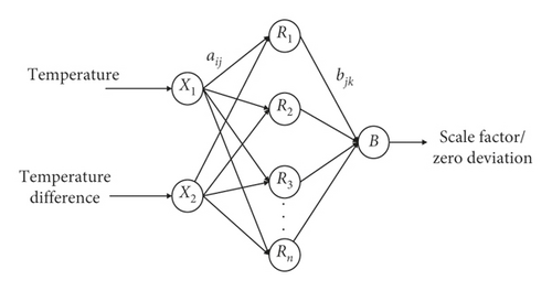
The corresponding transformation relationship of each layer is as follows.

Input layer to the hidden layer:

\begin{matrix} y_{i} = f ({net}_{j}), j = 1,2, \dots, m, \\ {net}_{j} = \sum_{i = 0}^{m} a_{i j} x_{i}, j = 1,2, \dots, m . \end{matrix}

(15)

Hidden layer to the output layer:

\begin{matrix} B_{k} = f ({net}_{k}), k = 1,2, \dots, l, \\ {net}_{k} = \sum_{j = 0}^{m} b_{j k} y_{j}, j = 1,2, \dots, l . \end{matrix}

(16)

Network error F:

\begin{matrix} F = \frac{1}{2} \sum_{i = 1}^{k} {\{d_{l} - f [\sum_{j = 0}^{l} b_{j k} f (\sum_{0}^{n} a_{i j} x_{i})]\}}^{2}, \end{matrix}

(17)

where x_i is the temperature and temperature difference of the input variable; a_ij and b_jk are the connection weights of each layer; B_k is the network output value of the scale factor and zero offset; d is the expected value of the scale factor and zero offset. The transfer functions f(x) are sigmoid function and linear transfer function purelin, respectively. The learning function accelerates the network convergence speed for the Levenberg–Marquardt algorithm, thus establishing a scale factor and zero-bias BP network model.

2.4.2. GA-BP Temperature Compensation Model

In view of the fact that genetic algorithm (GA) is a probabilistic adaptive iterative optimization process, it has good global search performance and is not easy to fall into local minimum. Even if the defined fitness function is discontinuous and irregular, it can find the overall optimal solution with the greatest probability. It is suitable for parallel processing. The search does not rely on the characteristics of gradient information. So, GA can be used to optimize the initial weight and threshold of BP neural network and search in a large range instead of the random selection of general initial weights. Then, the BP algorithm is used to fine-tune the network in the solution space to search for the optimal solution or approximate optimal solution. This not only achieves the complementary advantages of the two but also exerts the extensive nonlinear mapping ability of the neural network and the global search ability of the genetic algorithm. It accelerates the network learning speed and improves the approximation ability and generalization ability in the whole learning project [22].

(1)
Determining the sample number of input factor temperature, temperature difference, and output factor scale factor/zero deviation, and setting the fitness function, generate the weight value, and threshold value randomly to generate the initial population and code.
(2)
The network output of the corresponding chromosome is obtained through the network calculation of the scale factor and zero-deviation input sample.
(3)
Calculating the fitness of the chromosome using the fitness function.
(4)
Regenerating, crossing, and mutating to produce a new generation of population.
(5)
The termination condition is reached, and the global optimal network weight and threshold are obtained; otherwise, the above step (3) is returned.

The GA-BP temperature compensation model of the High-G MEMS accelerometer was completed by the above method.

The design flow chart of BP neural network optimization by GA is shown in Figure 2:

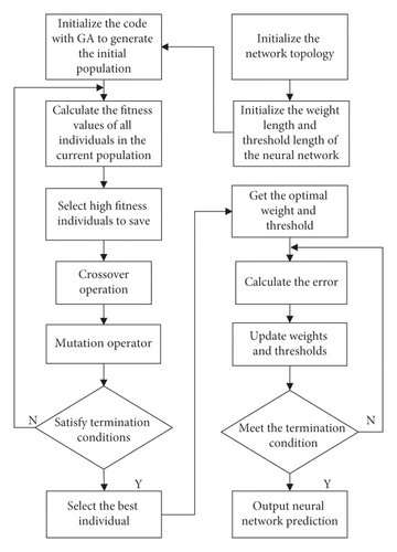
In this study, according to the empirical formula m = 2n + 1, the number of hidden layer nodes can be determined to be 5, where m is the number of hidden layer nodes and n is the number of input variables. The learning rate will affect the training times and network oscillation, so the learning rate Lr is 0.6 and the network accuracy is 0. 0001, thus completing the BP neural network structure parameter setting.

The size of the population determines the complexity of the chromosome. To adapt to chromosomal evolutionary ability, the group size is set to 30; the chromosome coding is in the binary form. A chromosome coding length of 15 is selected to improve the optimization efficiency. The advantages and disadvantages of the operator limit the search scope of the feasible domain. The law of survival of the fittest in nature is simulated. The roulette method is used to select the offspring. To truly reflect the impact of nature on populations, the crossover operator uses 0.7. To ensure population diversity to avoid malformation of the population which can affect the search mechanism, the crossover operator is set to 0.01. Thus, all of the parameters are set for the entire network model of GA-BP.

2.5. EMD, Wavelet Threshold, and Temperature Compensation Fusion Algorithm

When a signal has a very small useful signal amplitude and is largely annihilated by noise, using wavelet analysis for denoising is not ideal. The temporal and spatial filtering algorithm used in EMD simply removes one or more of the IMF components. It results in the deletion of corresponding useful signals. Therefore, EMD is a very approximate denoising method that can result in significant signal distortion. Here, we combine EMD with the wavelet thresholding to offset the respective disadvantages of each method. In addition, since the MEMS accelerometer is greatly affected by temperature, we include temperature compensation in the denoising method. In this paper, we combine EMD, wavelet thresholding, and temperature compensation into a single method. The algorithm for this method is given as follows:

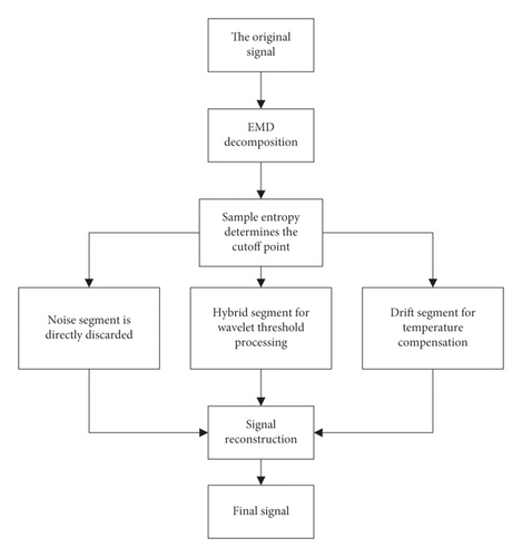
(1)
The original signal is decomposed by EMD to obtain the modal components
(2)
The SE algorithm is used to divide the IMF components into three segments: a noise segment, a mixing segment, and a drift segment
(3)
The noise segment is directly rounded off, the mixing segment is processed using wavelet thresholding, and temperature compensation is performed on the drift segment

The two segments perform signal reconstruction to obtain the final signal. The flow of the fusion algorithm is shown in Figure 3.

3. Structure and Structural Parameters of the High-G MEMS Accelerometer

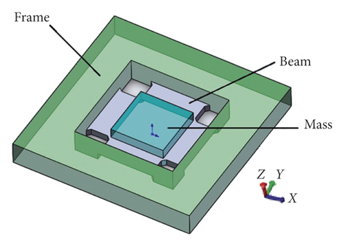
The original signal collected in this paper comes from a newly designed and manufactured High-G MEMS accelerometer [23]. Its structure is in the form of four-beam islands. The beam and mass are rectangular and easy to manufacture. The beam and mass structure are supported by a frame and connected to the bottom [24, 25]. Its structure diagram and size are shown in Figure 4.

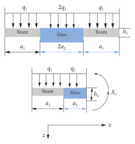
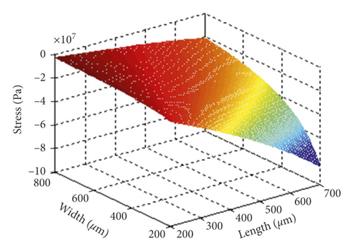
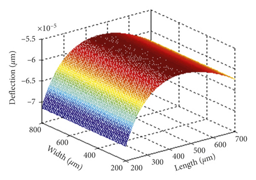
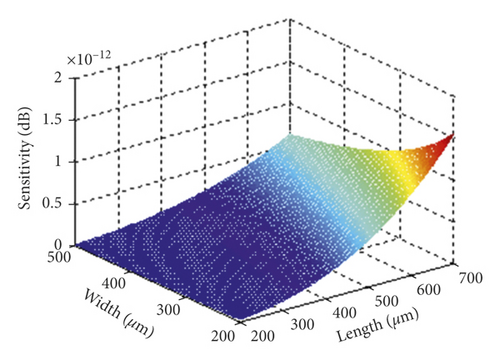
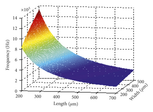
The length and width parameters of the beam were optimized using the MATLAB simulation method. The software is used to analyze the relationship between deflection, stress, mechanical sensitivity, and resonant frequency versus the length and width of the accelerometer. And Figure 5 is drawn. After comprehensive consideration of various factors, the structural parameters were modified and optimized, as shown in Table 1:

Table 1. Structural parameters of the High-G MEMS accelerometer.

	Mass			Beam
Parameters	Length (a₁)	Width (b₁)	Height (c₁)	Length (a₂)	Width (b₂)	Height (c₁)
Size (μm)	800	800	200	350	800	80

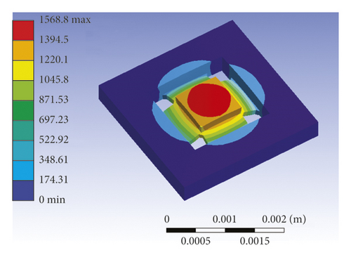
The first-order mode is simulated and analyzed by ANSYS software, as shown in Figure 6. The first mode mass moves along the Z axis, and its resonant frequency is 408 kHz, which is the working mode.

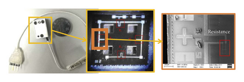
The structure of the High-G MEMS accelerometer is made of silicon and bonding on glass, and the SEM photos and CCD photos of the accelerometer structure are shown in Figure 7.

4. Experiment and Result Analysis

4.1. Temperature Experiment

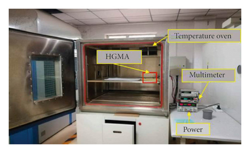
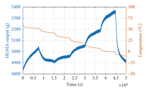
The equipment that is used in the temperature experiment consists of a temperature-controlled oven. A GWINSTEK GPS-4303C power supply provides a +5 V voltage to the High-G MEMS accelerometer, which is placed in the oven. The thermal resistance method is used to obtain the real-time temperature in the body of the accelerometer, and this value is synchronized with the High-G MEMS accelerometer output. The device is shown in Figure 8. The temperature of the oven can be accurately controlled from −50°C to +150°C. The temperature experiments are carried out over this range and high-speed data acquisition systems. Computers are used to collect the High-G MEMS accelerometer output signals. First, the temperature range on the oven is set from −10°C to 60°C. Then, data are collected continuously for the oven temperature and the output value of the accelerometer. The curves for these two data sets are shown in Figure 8.

4.2. Result Analysis

It can be seen from Figure 9 that the output of the accelerometer changes significantly with temperature. First, we use three noise reduction models to compensate for the output of the accelerometer in the temperature experiment: EMD, wavelet thresholding, and EMD + wavelet thresholding. The EMD decomposition diagram is shown in Figure 10. It is well known that these signals are characterized by high-frequency noise and low-frequency drift. Therefore, after the EMD decomposition is completed, the SE algorithm is used to calculate the SE values of the decomposed 15 IMF components. Then, the 15 IMF components are segmented by the SE values. The 15 IMF components are decomposed into three segments [26]. In this paper, based on the characteristics of the 15 IMF components, we analyze that the signal sequence with SE greater than 1 is very complicated. It contains a lot of noise and belongs to the noise segment. Between 0.2 and 1 is a mixed segment of noise and signal and less than 0.2 is a noiseless drift segment.

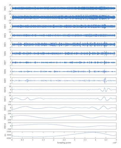
The first segment contains the first and second IMF components and is the noise segment C1; the second segment contains the third and fourth IMF components and is the mixing segment C2; and the third segment contains the fifth to fifteenth IMF components and is the drift segment C3, as shown in Figure 11.

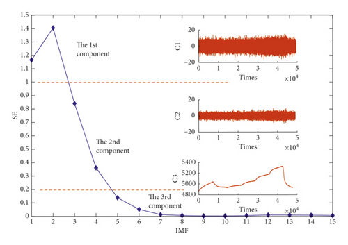
It can be seen from the Figure 11 that the noise segment is very rough, but the trend is stable. This indicate that this segment contains only a large amount of noise, and there is no drift phenomenon regardless of temperature. The mixing segment noise is significantly less than the noise segment but still contains noise. Its trend is smooth and there is no drift. The drift segment is no longer rough. We think it is only affected by temperature, causing drift and no noise.

After SE stratifies the signal, noise reduction models are developed. In EMD noise reduction, the first and second intrinsic mode functions are directly discarded because they are noise segments and are random and independent of temperature. The remaining components are used to reconstruct the signal. In wavelet threshold denoising, the “db5” wavelet is selected as the wavelet generating function. The decomposition scale is set to 5. And, wavelet threshold denoising is performed on the entire signal. In the EMD + wavelet thresholding method, the noise segment is discarded, the mixing segment is subjected to wavelet threshold processing, and the drift segment is left unchanged. Finally, the signal is reconstructed. The results from the three noise reduction models are shown in Figure 12.

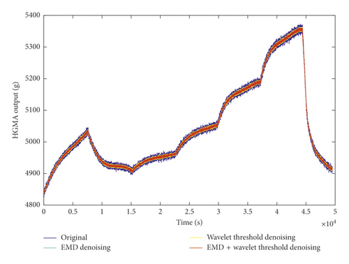
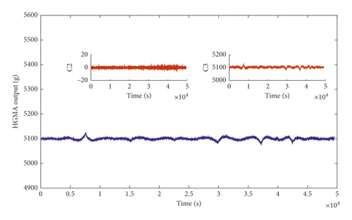
The results for each model are calculated. They show that all of the three models approximate the original data well. Of the three models, EMD and wavelet threshold have almost the same effect on noise suppression. The EMD + wavelet thresholding exhibits the best noise suppression. Then, using the results from noise reduction by the EMD + wavelet threshold method, GA-BP temperature compensation is implemented for the drift segment of the signal. So, an EMD + wavelet thresholding + (GA-BP) temperature compensation model is developed. Finally, C2 and C3 are reconstructed to obtain the final signal, as shown in Figure 13.

Allan variance [27, 28]is used to evaluate the noise reduction effect and temperature compensation effect of the four methods (Figure 14).

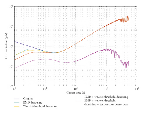
The results for the acceleration random walk (which represents the noise characteristics) and zero-bias stability are shown in Table 2. The data show that the values for the acceleration random walk that are obtained using the EMD, wavelet thresholding, and EMD + wavelet thresholding methods are 338.184 g/h/Hz^0.5, 338.02 g/h/Hz^0.5, and 207.518 g/h/Hz^0.5, respectively. The corresponding values for the zero-deviation stability are 49275.9 g/h, 49274.7 g/h, and 49275.5 g/h, respectively. When temperature compensation is added, the values for the acceleration random walk and the zero-bias stability are 79.15 g/h/Hz^0.5 and 774.7 g/h, respectively. It indicates that the accelerometer noise has been sufficiently suppressed and the temperature drift has been well compensated for. The main content of this paper is to propose a new signal processing method, which is a software processing method. The limitation of this method is that it cannot be processed in real time and must be completely collected before processing. Processing speed depends on how fast the computer software is running. The faster the computer runs, the faster the results will be processed. Our goal is to provide a more efficient signal processing method for the same or similar scholars refer to. In the future, we will continue to strengthen research in this field and strive to develop more effective and effective methods.

Table 2. Results of Allah’s analysis of variance.

Denoising				Temperature Compensation
Original data	EMD	Wavelet	EMD + wavelet	EMD + wavelet
B(g/h/Hz^0.5) N(g/h)	B(g/h/Hz^0.5) N(g/h)	B(g/h/Hz^0.5) N(g/h)	B(g/h/Hz^0.5) N(g/h)	B(g/h/Hz^0.5) N(g/h)
1712.66	338.184	338.02	207.518	79.15
49275	49275.9	49274.7	49275.5	774.7

5. Conclusion

In this paper, a fusion algorithm of EMD + wavelet thresholding + (GA-BP) temperature compensation is studied to improve the accuracy of a newly developed High-G accelerometer. The fusion algorithm first performs EMD decomposition on the original accelerometer signal to obtain IMF components. Then, IMF components are segmented by SE. The noise segment is directly omitted, wavelet thresholding is performed on the mixing segment, and a GA-BP performs temperature compensation on the drift segment. Finally, signal reconstruction is implemented. In the fourth part of this paper, EMD, wavelet thresholding, EMD + wavelet thresholding, and EMD + wavelet thresholding + temperature compensation results are compared by Allan variance calculation. And, the fusion algorithm is found to be the best. As shown by data, the acceleration random walk and zero-deviation stability change from 1712.66 g/h/Hz^0.5 and 49275 g/h to 79.15 g/h/Hz^0.5 and 774.7 g/h, respectively. This indicates that the fusion algorithm not only effectively suppresses the noise but also compensates for temperature drift in the accelerometer.

Conflicts of Interest

The authors declare that they have no conflicts of interest.

Acknowledgments

This work was supported by the National Natural Science Foundation of China (Nos. 51705477, 61703098, and 61603353) and Pre-Research Field Foundation of Equipment Development Department of China (No. 61405170104). This research was also supported by Top Young Academic Leaders of Higher Learning Institutions of Shanxi, Fund Program for the Scientific Activities of Selected Returned Overseas Professionals in Shanxi Province, Shanxi Province Science Foundation for Youths (No. 201801D221195), Young Academic Leaders of North University of China (No. QX201809), Open Fund of State Key Laboratory of Deep Buried Target Damage (No. DXMBJJ2017-15), and Fund for Shanxi “1331 Project” Key Subjects Construction.

Open Research

Data Availability

The data used to support the findings of this study are available from the corresponding author upon request.

References

1 Liu Y. and Ma T., Parasitic resistance-based high precision capacitive MEMS accelerometer phase shift and its usage for temperature compensation, IEEE Sensors Journal. (2018) 18, no. 2, 629–634, https://doi.org/10.1109/jsen.2017.2777864, 2-s2.0-85035810825.
10.1109/JSEN.2017.2777864
CAS Web of Science® Google Scholar
2 Lu Q., Pang L., Huang H. et al., High-G calibration denoising method for high-G MEMS accelerometer based on EMD and wavelet threshold, Micromachines. (2019) 10, no. 2, https://doi.org/10.3390/mi10020134, 2-s2.0-85061720433.
10.3390/mi10020134
Web of Science® Google Scholar
3 Shen C., Yang J., Tang J., Liu J., and Cao H., Parallel processing algorithm of temperature and noise error for micro-electro-mechanical system gyroscope based on variational mode decomposition and augmented nonlinear differentiator, Review of Scientific Instruments. (2018) 89, no. 7, 076107, https://doi.org/10.1063/1.5037052, 2-s2.0-85050717382.
10.1063/1.5037052
PubMed Web of Science® Google Scholar
4 Wang Z., Du W., Wang J. et al., Research and application of improved adaptive MOMEDA fault diagnosis method, Measurement. (2019) 140, 63–75, https://doi.org/10.1016/j.measurement.2019.03.033.
10.1016/j.measurement.2019.03.033
Web of Science® Google Scholar
5 Cao H., Li H., Liu J., Shi Y., Tang J., and Shen C., An improved interface and noise analysis of a turning fork microgyroscope structure, Mechanical Systems and Signal Processing. (2016) 70-71, 1209–1220, https://doi.org/10.1016/j.ymssp.2015.08.002, 2-s2.0-84953938644.
10.1016/j.ymssp.2015.08.002
Web of Science® Google Scholar
6 Wang W. and Liu L., Fourier transform and valuations, Journal of Mathematical Analysis & Applications. (2019) 470, no. 2, 1167–1184, https://doi.org/10.1016/j.jmaa.2018.10.056, 2-s2.0-85055205269.
10.1016/j.jmaa.2018.10.056
Web of Science® Google Scholar
7 Li R., Wang J., and Chen Y., Effect of the signal filtering on detrended fluctuation analysis, Physica A: Statistical Mechanics and Its Applications. (2018) 494, 446–453, https://doi.org/10.1016/j.physa.2017.12.011, 2-s2.0-85038838042.
10.1016/j.physa.2017.12.011
Web of Science® Google Scholar
8 Wang Z., He G., Du W. et al., Application of parameter optimized variational mode decomposition method in fault diagnosis of gearbox, IEEE Access. (2019) 7, no. 7, 44871–44882, https://doi.org/10.1109/access.2019.2909300.
10.1109/ACCESS.2019.2909300
Web of Science® Google Scholar
9 Lazhari M. and Sadhu A., Decentralized modal identification of structures using an adaptive empirical mode decomposition method, Journal of Sound and Vibration. (2019) 447, 20–41, https://doi.org/10.1016/j.jsv.2019.01.049, 2-s2.0-85061065201.
10.1016/j.jsv.2019.01.049
Web of Science® Google Scholar
10 Bi F., Ma T., and Wang X., Development of a novel knock characteristic detection method for gasoline engines based on wavelet-denoising and EMD decomposition, Mechanical Systems and Signal Processing. (2019) 117, 517–536, https://doi.org/10.1016/j.ymssp.2018.08.008, 2-s2.0-85051706677.
10.1016/j.ymssp.2018.08.008
Web of Science® Google Scholar
11 Yang G., Dai J., Liu X., Wu X., Chen M., and Qin H., Denoising of gamma-ray spectrum by optimized wavelet thresholding based on modified genetic algorithm in carbon/oxygen logging, Journal of Radioanalytical and Nuclear Chemistry. (2019) 320, no. 2, 351–359, https://doi.org/10.1007/s10967-019-06477-x, 2-s2.0-85063205496.
10.1007/s10967-019-06477-x
CAS Web of Science® Google Scholar
12 Cao H., Zhang Y., Shen C., Liu Y., and Wang X., Temperature energy influence compensation for MEMS vibration gyroscope based on RBF NN-GA-KF method, Shock And Vibration. (2018) 2018, 10, 2830686, https://doi.org/10.1155/2018/2830686, 2-s2.0-85058947311.
10.1155/2018/2830686
Web of Science® Google Scholar
13 Shen C., Liu X., Cao H. et al., Brain-like navigation scheme based on MEMS-INS and place recognition, Applied Sciences. (2019) 9, no. 8, https://doi.org/10.3390/app9081708.
10.3390/app9081708
Google Scholar
14 Cao H., Zhang Y., Han Z. et al., Pole-zero temperature compensation circuit design and experiment for dual-mass MEMS gyroscope bandwidth expansion, IEEE/ASME Transactions on Mechatronics. (2019) 24, no. 2, 677–688, https://doi.org/10.1109/TMECH.2019.2898098.
10.1109/TMECH.2019.2898098
Web of Science® Google Scholar
15 Shrivastava Y. and Singh B., A comparative study of EMD and EEMD approaches for identifying chatter frequency in CNC turning, European Journal of Mechanics-A/Solids. (2019) 73, 381–393, https://doi.org/10.1016/j.euromechsol.2018.10.004, 2-s2.0-85054867536.
10.1016/j.euromechsol.2018.10.004
Web of Science® Google Scholar
16 Akkar H. A. R., Hadi W. A. H., and Al-Dosari I. H. M., Implementation of sawtooth wavelet thresholding for noise cancellation in one dimensional signal, International Journal of Nanoelectronics & Materials. (2019) 12, no. 1, 67–73.
Web of Science® Google Scholar
17 Zhao S., Wang C., and Bian X., Research on harmonic detection based on wavelet threshold and FFT algorithm, Systems Science & Control Engineering. (2018) 6, no. 3, 339–345, https://doi.org/10.1080/21642583.2018.1558420, 2-s2.0-85062605090.
10.1080/21642583.2018.1558420
Google Scholar
18 Wang Z., Zhou J., Wang J. et al., A novel fault diagnosis method of gearbox based on maximum kurtosis spectral entropy deconvolution, IEEE Access. (2019) 7, 29520–29532, https://doi.org/10.1109/access.2019.2900503.
10.1109/ACCESS.2019.2900503
Web of Science® Google Scholar
19 Petersen K. and Wilson B., Dynamical intricacy and average sample complexity, Dynamical Systems. (2018) 33, no. 3, 369–418, https://doi.org/10.1080/14689367.2017.1374352, 2-s2.0-85029707590.
10.1080/14689367.2017.1374352
Google Scholar
20 Raffalt P. C., McCamley J., Denton W., and Yentes J. M., Sampling frequency influences sample entropy of kinematics during walking, Medical & Biological Engineering & Computing. (2019) 57, no. 4, 759–764, https://doi.org/10.1007/s11517-018-1920-2, 2-s2.0-85055684183.
10.1007/s11517-018-1920-2
PubMed Web of Science® Google Scholar
21 Fang P., Cai Z., and Zhang P., Application of the GA-BP neural network in earthwork calculation, IOP Conference Series: Materials Science and Engineering. (2018) 301, no. 1, https://doi.org/10.1088/1757-899x/301/1/012130, 2-s2.0-85045265299.
10.1088/1757-899X/301/1/012130
Google Scholar
22 Guo N., Fang Y., Tian Z., and Cao S., Research on SOC fuzzy weighted algorithm based on GA-BP neural network and ampere integral method, The Journal of Engineering. (2019) 2019, no. 15, 576–580, https://doi.org/10.1049/joe.2018.9385.
10.1049/joe.2018.9385
Web of Science® Google Scholar
23 Shi Y., Yang Z., Ma Z. et al., The development of a dual-warhead impact system for dynamic linearity measurement of a high-g micro-electro-machanial-system (MEMS) accelerometers, Sensors. (2016) 16, no. 6, 582–593, https://doi.org/10.3390/s16060840, 2-s2.0-84973480931.
10.3390/s16060840
Web of Science® Google Scholar
24 Shi Y., Zhao Y., Feng H. et al., Design, fabrication and calibration of a high-G MEMS accelerometer, Sensors & Actuators: A. Physical. (2018) 279, 733–742, https://doi.org/10.1016/j.sna.2018.07.010, 2-s2.0-85049893266.
10.1016/j.sna.2018.07.010
CAS Web of Science® Google Scholar
25 Cao H., Li H., Shao X. et al., Sensing mode coupling analysis for dual-mass MEMS gyroscope and bandwidth expansion within wide-temperature range, Mechanical Systems and Signal Processing. (2018) 98, 448–464, https://doi.org/10.1016/j.ymssp.2017.05.003, 2-s2.0-85022200132.
10.1016/j.ymssp.2017.05.003
Web of Science® Google Scholar
26 Shen C., Li J., Zhang X., Tang J., Cao H., and Liu J., Multi-scale parallel temperature error processing for dual-mass MEMS gyroscope, Sensors and Actuators A: Physical. (2016) 245, 160–168, https://doi.org/10.1016/j.sna.2016.04.055, 2-s2.0-84966444579.
10.1016/j.sna.2016.04.055
CAS Web of Science® Google Scholar
27 Guo H., Chen Y., Wu D. et al., Plasmon-enhanced sensitivity of spin-based sensors based on a diamond ensemble of nitrogen vacancy color centers, Optics Letters. (2017) 42, no. 3, 403–406, https://doi.org/10.1364/ol.42.000403, 2-s2.0-85011653958.
10.1364/OL.42.000403
CAS PubMed Web of Science® Google Scholar
28 Guo H., Zhu Q., Tang J. et al., A temperature and humidity synchronization detection method based on microwave coupled-resonator, Sensors and Actuators B: Chemical. (2018) 261, 434–440, https://doi.org/10.1016/j.snb.2018.01.142, 2-s2.0-85041421995.
10.1016/j.snb.2018.01.142
CAS Web of Science® Google Scholar

Citing Literature

All articles

Fusion Algorithm-Based Temperature Compensation Method for High-G MEMS Accelerometer

Abstract

1. Introduction