In this study, the optimization of a low-speed wing with functional constraints is discussed. The aerodynamic analysis tool developed by the coupling of the numerical nonlinear lifting-line method to Xfoil is used to obtain lift and drag coefficients of the baseline wing. The outcomes are compared with the results of the solver based on the nonlinear lifting-line theory implemented into XLFR5 and the transition shear stress transport model implemented into ANSYS-Fluent. The agreement between the results at the low and moderate angle of attack values is observed. The sequential quadratic programming algorithm of the MATLAB optimization toolbox is used for the solution of the constrained optimization problems. Three different optimization problems are solved. In the first problem, the maximization of is the objective function, while level flight condition at maximum is defined as a constraint. The functional constraints related to the wing weight, the wing planform area, and the root bending moment are added to the first optimization problem, and the second optimization problem is constructed. The third optimization problem is obtained by adding the level flight condition and the available power constraints at the maximum speed and the level flight condition at the minimum speed of the baseline unmanned air vehicle to the second problem. It is demonstrated that defining the root bending moment, the wing area, and the available power constraints in the aerodynamic optimization problems leads to more realistic wing planform and airfoil shapes.

1. Introduction

Recent advances in computer technology have advanced the conceptual design of an aircraft using advanced optimization tools rather than rough sketches and calculations on paper. In the early years of aviation, a small group of engineers, led by a design engineer who had experience in both design and manufacturing, were responsible for the conceptual design. However, at present, the design group has expanded and divided into subgroups because of the complexity of the aircraft, which is a result of the technological advances [1]. Simultaneously, faster solutions of the optimization problems have enabled the definition of optimization problems that have objective functions and constraints defined by different disciplines to satisfy the expected performance merits of the aircraft in the conceptual design. In addition to satisfying the performance merits, developing a mathematical proof of the optimized aircraft at the end of the design phase is crucial. To obtain accurate results in the optimization problems, the function evaluator should be a verified and widely used analytical or numerical analysis tool.

Xfoil, developed by Mark Drela, is utilized as the airfoil analysis code in the numerous studies that are related to the design of fixed and rotary wings, wind turbine blades, and marine propellers [2]. Aerodynamic coefficients are obtained by the coupling of the panel method to the two-equation integral boundary-layer formulation that is the integral momentum and kinetic energy shape parameter equations. Falkner-Skan and Swafford velocity profile formulas are used for laminar closure and turbulent closure, respectively. The eⁿ method is implemented for transition point detection [3].

Koreanschi et al. used Xfoil for the evaluation of the base airfoil performance in their study that presented numerical optimization and experimental wind tunnel testing of a morphing wing tip equipped with an adaptable upper surface, and a rigid aileron [4]. Gabor et al. used Xfoil in the high angle of attack (α) optimization of a morphing airfoil as a function evaluator [5]. Della Vecchia et al. investigated the effect of a morphing trailing edge to the performance of a high-altitude long-endurance (HALE) aircraft. The variation of the lift coefficient (C_l) and the profile drag coefficient (C_d) of the airfoils with trailing edge deflection was obtained with Xfoil [6]. Magrini and Benini investigated the aerodynamic optimization of a morphing leading-edge airfoil. The optimization problem was solved by using the transition SST model, Spalart-Allmaras model, and Xfoil [7]. Liu et al. studied the optimization of the airfoil at an ultra-low Reynolds number (Re) for nanorotor performance [8]. In the study, Xfoil results were compared with the results of a two-dimensional incompressible Navier-Stokes solver in which the artificial compressibility method was utilized to deal with incompressible flow. In this validation study, the National Advisory Committee for Aeronautics (NACA) 0006 airfoil was used and Re was 6000. Xfoil captured C_l and C_d values up to stall α correctly. Silvestre et al. coupled the blade element momentum theory with Xfoil and developed a new propeller design code named as JBLADE [9].

The nonlinear numerical lifting-line method proposed by Anderson and Corda is an iterative solution to Prandtl’s lifting-line theory [10]. Gamboa et al. used the nonlinear lifting-line method as a function evaluator for the morphing wing optimization. In the study, airfoil aerodynamic data was provided by Xfoil [11]. Merz et al. used the numerical nonlinear lifting-line method to find the most effective α on a pitching rotor blade [12].

2. Method

First of all, this paper describes the coupling of the nonlinear numerical lifting-line method to Xfoil. Then, the results of the newly designed aerodynamic analysis tool are compared with the results of the solver based on the nonlinear lifting-line theory (LLT) implemented into XLFR5 and the transition (γ − Re_θ) shear stress transport (SST) model implemented into ANSYS-Fluent. After that, three different optimization problems in which maximization is the objective function are constructed. The optimization problems are defined by adding new functional constraints that are the wing root bending moment (M_b), the wing weight (W_w), the wing planform area (S), the level flight condition and power available (P_A) at the maximum speed (V_max), and the level flight condition at the stall speed (V_stall) of the baseline unmanned air vehicle (UAV). The change of the objective function, the constraints, the wing planform, and the airfoil shapes is discussed. This study differs from the studies in the literature because the performance of the UAV at both V_max and V_stall conditions at the level flight is taken into account with the functional constraints in the optimization problems that are discussed below.

2.1. The Nonlinear Numerical Lifting-Line Theory

In this part of the study, the methodology of the nonlinear numerical lifting-line theory and integration of Xfoil to it are discussed. The numerical solution starts with the division of the span (b) of the finite wing into N number of spanwise stations in the y-direction as shown in Figure 1 [13]. In Figure 1, the distance between the equidistant stations is Δy. The method needs an initial circulation distribution (Γ(y)) along the span. The elliptic circulation distribution in equation (1) is acceptable for this requirement.

(1)

Details are in the caption following the image — **Figure 1**
Open in figure viewer PowerPoint

The positions of the stations.

In the above equation, Γ₀ is the circulation at the root chord (c_r). By using initial Γ(y), the induced angle of attack (α_i) for the n^th panel is obtained as follows:

(2)

This integral is evaluated numerically by using Simpson’s rule [13]:

(3)

where V_∞ is the freestream velocity. For the calculation of α_i, dΓ/dy is needed. Although dΓ/dy is analytically available for the initial calculation [13], as shown in equation (4), it must be calculated by using a finite difference method for the other iterations as shown in equation (5).

The forward difference method is selected for the process.

(4)

(5)

In order to avoid singularity when y_n = y_j−1, y_j, or y_j+1, the average of the neighbor stations’ results is taken as the result of the corresponding term [13]. After the calculation of α_i, the effective angle of attack (α_eff) is obtained by subtracting α_i from the geometric angle of attack (α_geo).

(6)

At this point, it should be stated that the method is a numerical iterative solution to Prandtl’s lifting-line theory that states that the circulation is zero when y = ±b/2 [14]. That implies that C_l values of the airfoils at the tip chords (c_t) of the wing are zero and α_eff is equal to zero lift angle of attack value

of the airfoils at the tips as shown in

(7)

Once α_eff distribution along the span is known, C_l and C_dof the airfoils at the stations are calculated by using Xfoil [15]. An interface developed to run Xfoil in MATLAB is used [16]. It is modified for the MAC OSX operating system. Then, the new circulation distribution (Γ_new) is calculated by using

(8)

c(y) in the above equation is the chord value at the station. The input circulation values are calculated by using a damping factor (D) as follows:

(9)

The iterative solution requires a strong damping factor. Setting D values as one leads to divergent iteration [10]. The iteration process stops if the Euclidean norm of the difference between the new circulation vector and the input circulation vector is less than a convergence criterion (ε):

(10)

By using converged circulation distribution, the lift (L) [10], the induced drag (D_i) [10], and the root bending moment (M_b) [17] of the wing are calculated as follows:

(11)

(12)

(13)

where ρ_∞ is the free stream density. These integrals are also evaluated numerically by using Simpson’s rule. The parasite drag of the wing (D_pr) is calculated by using

(14)

After the calculations of the aerodynamic forces and moments, the lift coefficient (C_L), the drag coefficient (C_Dw), and the root bending moment coefficient (C_Mb) of the wing are obtained as follows:

(15)

(16)

(17)

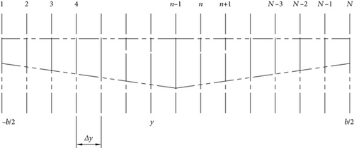
As a result, Xfoil and the numerical nonlinear lifting-line method are coupled and the aerodynamic analysis tool is obtained.

2.2. XFLR5 LLT and ANSYS-Fluent γ − Re_θ SST Model

The XFLR5 LLT and ANSYS-Fluent γ − Re_θ SST model are introduced in this section. XFLR5 is an analysis tool for airfoils and wings. There are four different solvers based on the solution of the inviscid potential flow implemented into it. These are the solvers based on the horseshoe vortex lattice method, the ring vortex lattice method, the 3-D panel method, and the nonlinear lifting-line theory. They were used to calculate the drag polar of the different wings [18–20].

The solver based on nonlinear lifting-line theory calculates the C_L and C_Dw results by taking the drag polar data of the airfoil form Xfoil that is also implemented into XFLR5. The results are obtained by using the default values defined from the solver except for the iteration number. It is set to 1000.

Another computational fluid dynamics (CFD) tool, ANSYS-Fluent, which solves the problems according to the finite volume method, is used to compare the C_L and C_Dw results obtained by the aerodynamic analysis tool.

Langtry and Menter developed a new correlation-based transition model to simulate laminar to turbulent transition [21]. The model is essentially based on two transport equations. One equation is for a transition onset criterion and the other is for intermittency. To validate this model, they gave examples of the cases which they studied such as 2-D three-element flap, 2-D airfoil, and a transonic wing. They stated that the transitional CFD simulation was in very good agreement with the experimental results. Aftab et al. compared the following turbulence models for the flow over the NACA4415 airfoil for Re of 120000 with the experimental results: Spalart-Allmaras, K − ω SST, intermittency SST, k − kl − ω, and γ − Re_θ SST [22]. According to the results, only the γ − Re_θ SST provided reliable results for low and high α values. Lanzafame et al. developed a horizontal axis wind turbine 3-D CFD model to predict wind turbine performance [23]. They compared K − ω SST and γ − Re_θ SST with experimental data. According to the result, γ − Re_θ SST captured the trend of the aerodynamic coefficients whereas K − ω SST overpredicted C_l values and underpredicted C_d values.

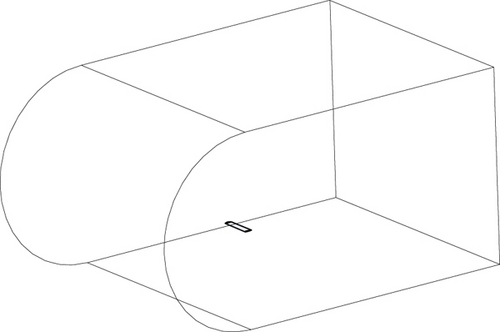
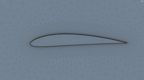
According to these studies in the literature, the computations are performed with γ − Re_θ SST in this study. The numerical studies are carried out according to the pressure-based method. There are some specific criteria that determine the accuracy of the results obtained with ANSYS-Fluent. The first is to determine the size of the boundary region where flow analysis is intended. For this study, the size of the boundary is formed approximately 30 times larger than the maximum wing thickness and wing chord length as shown in Figure 2 [24, 25]. Since the control volumes are 3-D, the volumetric adaptation of the inflation layers and the prism cells are used. The dimensionless distance to the wall (y⁺) is selected as 1 [26]. Thereby, first-layer height is calculated as 0.015 mm for the selected y⁺. The growth rate and the number of inflation layers are selected as 1.1 and 61, respectively. These selections create a mesh with 2569785 elements and with a maximum skewness value of 0.95 as shown in Figure 3. The turbulence intensity is selected as 1%. For the convergence criterion, the continuity equation is evaluated as 2 · 10⁻⁴ for 0° α. In order to provide convergence, approximately 1600 iterations are performed. The convergence criterion for high α values increases up to 10 times. Therefore, the results are accepted as accurate in these calculations when fluctuations in C_L and C_Dw lie within the range of ±0.001.

2.3. Comparison of the Aerodynamic Analysis Tool with ANSYS-Fluent

The comparison of the aerodynamic analysis tool with XFLR5 6.47 LLT and the ANSYS-Fluent 16.2 γ − Re_θ SST model is made in this part of the paper. The flow solutions of the aerodynamic analysis tool are obtained on a 2.4 GHz Intel Core i7, 8 GB MacBook Pro. The computation of ANSYS-Fluent is performed on 2 processors of 2.4 GHz Intel Xeon E5, 32 GB HP Z820.

The interface is modified so that C_l and C_d values are obtained for the airfoils at each station by parallel processing. When Xfoil fails to converge, the initial panel number, which is 200, is altered between 194 and 206. NACA 4412 airfoil with closed trading edge is used as the candidate airfoil. Equations (18) and (19) are used for the half thickness (z_t) and the camber generation (z_c), respectively. In these equations, t is the maximum thickness in hundredths of the chord, p is the maximum camber location in tenths of the chord, and m is the maximum camber in hundredths of the chord. x coordinates are generated by the cosine distribution.

The z coordinates of the upper surface are obtained by summing equations (18) and (19), whereas equation (18) is subtracted from equation (19) for the lower surface as is done in the NACA airfoil generation subroutine of Xfoil [27].

(18)

(19)

c_r, c_t, and b are 0.45 m, 0.45 m, and 4 m, respectively. ρ_∞ is 1.225 kg/m³. The dynamic viscosity (μ_∞) is 1.7974 · 10⁻⁵ Ns/m² and V_∞ is 22 m/s. In Xfoil, the default critical n value of the eⁿ transition prediction method is nine. This value is changed as 2.62, because it corresponds to the selected turbulent intensity in the ANSYS-Fluent analysis.

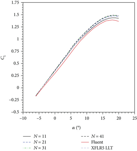
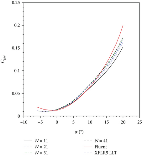
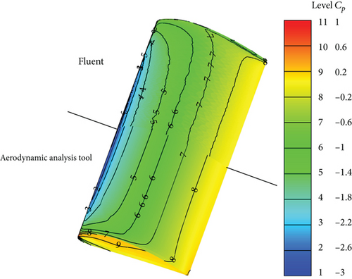
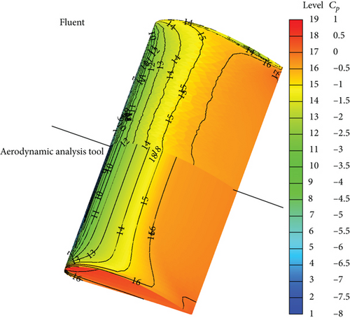
In Figure 4, the C_L results for the different panel station numbers and the results of ANSYS-Fluent and XFLR5 are shown. According to the results in Figure 4, ANSYS-Fluent calculates the least C_L at the same α. C_L values of N = 21, N = 31, and N = 41 cases overlap. The results show slight difference with the results of XFLR5 LLT and capture the trend line of ANSYS-Fluent up to the stall α. C_Dw values of ANSYS-Fluent are almost identical to N = 11 case values when α is between 0° and 10° as depicted in Figure 5. But as α gets close to 15°, the ANSYS-Fluent, N = 31 case, and N = 41 case yield similar C_Dw. After 15°, ANSYS-Fluent results start to diverge from the results of the aerodynamic tool. In order to investigate the situation in detail, the flow field around the wing for 10° and 18° α values is presented in Figures 6–9.

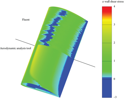
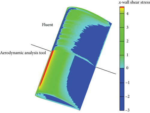
In the aerodynamic analysis tool, the transition region can be determined by finding the region at which a sudden increase in the x-wall shear stress is observed. The turbulent region is the region at which the x-wall shear stress values get closer to zero. Contrary to this, the transition region and the turbulent separation region are identified when x-wall shear stress is less than zero in the results of ANSYS-Fluent [28].

According to the results for 10°, apart from the slight difference around the leading edge, pressure contours are almost identical for both solvers as shown in Figure 6. The transition prediction by the aerodynamic solver is understood from the color change from green to yellow in Figure 7. ANSYS-Fluent captures the transition location almost at the same position as the aerodynamic analysis tool does that is shown by a color change from green to blue. Both solvers capture the separation around the trailing edge. When the results for 18° are discussed, one can easily see the difference between the pressure contours especially on the aft of the wing as depicted in Figure 8. As is shown in Figure 9, both solvers predict the transition region almost at the same location. ANSYS-Fluent predicts the turbulent separation ahead. But it is very close to the turbulent separation location of the aerodynamic analysis tool.

Since N = 31 and N = 41 cases capture the C_Dw values of ANSYS-Fluent at high α values, they are selected as the candidate station numbers.

In order to select the optimum N, D, and ε values, the total solution time (t_tot) to obtain drag polar results between the α values of -6° and 20° is compared for the different N, D, and ε values in Table 1. The maximum deviations in C_L(∆C_L) and C_Dw(∆C_Dw) are obtained with respect to the results when the N, D, and ε values are equal to 41, 0.05, and 0.01, respectively. According to the results, choosing the N value as 31 saves the computation time approximately by 38% at the same D and ε values when it is compared with the result of N = 41.

Table 1. Effect of N, D, and ε to the results and t_tot.

N	D	ε	∆C_L (%)	∆C_Dw (%)	t_tot (s)
41	0.05	0.01	0	0	3007.7
31	0.05	0.01	0.4	1.1	2532.9
31	0.1	0.01	0.4	1.1	1096.2
31	0.2	0.01	0.4	1.1	519.3
31	0.2	0.05	5.9	1.1	418.5
31	0.2	0.1	11.2	1.0	414.3
31	0.2	0.2	15.2	0.9	347.6

Increasing D decreases the computation time by 86.9% without boosting ∆C_L and ∆C_Dw. When D is selected as 0.4 and above, the convergence problem is observed at the high α values. Contrary to this, increasing ε yields drastic increase in ∆C_L especially at the negative α and the high α values. Apart from this region, ∆C_L is around 1% at the low α and moderate α values. In light of this information, N, D, and ε values are selected as 31, 0.2, and 0.01, respectively. t_tot of ANSYS- Fluent results is approximately 120 hours.

2.4. Optimization Solver

In this part, the advantages of the selected optimization solver and its use are discussed. Vanderplaats compared different optimization methods by using a structural optimization problem [29]. In the problem, the objective function was the minimization of the structural volume of a cantilevered beam that was fixed at the right end and had a vertical load applied at the free left end. The cantilevered beam had five segments and thicknesses, and heights of the segments were the design variables. In the study, the allowable bending stress at the right end of each segment was defined as the constraints. In addition to this, the allowable left end deflection was also defined as the constraint. The ratio of the height to the thickness of each segment was limited by using constraints. In summary, the identified optimization problem had 10 design variables and 11 constraints. Genetic search, sequential linear programming, method of feasible directions, generalized reduced gradient method, modified feasible directions method, and sequential quadratic programming (SQP) were compared in the study. The first method is an evolutionary optimization method whereas the others are the gradient-based optimization methods. The optimum results obtained by the methods were very close to each other. The genetic search method obtained the optimum result after 10⁶ function evaluations. Among the gradient-based optimization methods, SQP had the least number of iterations and the least number of gradient evaluations. The total number of function call is 125 for the SQP analysis. As discussed above, the main advantage of SQP is that it does not attempt to satisfy constraints at each iteration that results in less number of function calls [30]. Therefore, the SQP algorithm is used as given in the MATLAB optimization toolbox for the solution of the optimization problems that are discussed below.

The procedure for the optimization process is represented in Figure 10.

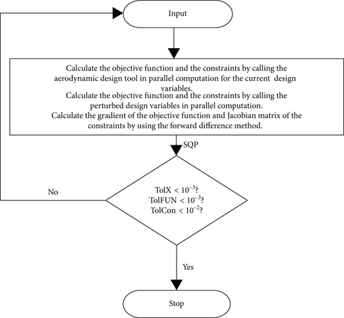
The design variable array is used to calculate the objective function and the constraints for the current step. For this case, the aerodynamic design tool is called in parallel computations and the threads are used to calculate C_l and C_d values for the airfoils at each station. After that, the design variable array is perturbed by an increment array that is 1% of each design variable array element. Parallel computing is applied for the calculation of the objective function and the constraints by using perturbed design variable array elements. The aerodynamic design tool runs in serial for this case. The forward difference method is used for the calculation of the gradient of the objective function and Jacobian matrix of the constraints.

The process stops if the change of the design variable array (TolX) or the change in the objective function (TolFun) is less than 10⁻³. The violation of the constraints (TolCon) is limited to 10⁻².

2.5. The Characteristics of the Baseline UAV

Before going into the details of the optimization problems, the geometric and performance characteristics of the baseline UAV and basic assumptions related to it are revealed in this part of the work. The baseline UAV is a propeller-driven aircraft and P_A of the engine is 2000 W. The drag coefficient of the other components (C_Doth) of the UAV except the wing is assumed as a varying parameter as follows:

(20)

where S_b is the planform area of the wing of the baseline UAV. As a result, the total drag coefficient (C_D) of the baseline UAV is the summation of C_Doth and C_Dw. The total weight of the UAV except for the wing (W_oth) is 250 N. The wing weight (W_w) is calculated as follows [31]:

(21)

where

denotes the wing mean aerodynamic chord, (t/c)_max the maximum thickness of the airfoil, AR the aspect ratio, and λ the taper ratio. ρ_mat is the density of the construction material that is graphite/epoxy. K_ρ is the wing density factor. They are selected as 1575 kg/m³ and 0.0016, respectively, by calculating the average values in the appropriate reference tables for homebuilt aircraft [31]. The relation between ultimate load factor (n_ult) and maximum positive load factor (n_max) is defined as follows:

(22)

Unlike a fighter aircraft, the producible n_max by the engine power is less than the tolerable n_max by the aircraft structure for a general aviation aircraft [32]. For this reason, the equation of the producible n_max by the engine power for the propeller-driven aircraft that is in equation (23) is used in the W_w calculation.

(23)

As seen in the above equations, W_w and n_max are implicit. The secant method is applied to find W_w.

The geometric parameters of the wing of the baseline UAV are shown in Table 2.

Table 2. Geometric properties of the baseline UAV’s wing.

Airfoil	NACA 4412
c_r	0.45 m
c_t	0.45 m
b	4
S_b	1.8 m²

The wing of the baseline UAV is a rectangular and unswept wing. The airfoil profile is constant along the span. Table 3 depicts the performance parameters of the baseline UAV.

Table 3. Performance parameters of the baseline UAV.

	14.08
α at	8°
V at	15.52 m/s
M_b at	127.46 Nm
W_w	24.06 N
V_max	39.45 m/s
α at V_max	-2.32°
V_stall	13.25
α at V_stall	18°

It has a maximum ratio of 14.08 when α is 8° and speed is 15.52 m/s. M_b is 127.46 Nm for this flight condition. W_w is 24.06 N. V_max is 39.45 m/s when α is -2.32° and V_stall is 13.25 m/s when α is 18^°.

3. Results

First of all, the details of the optimization problems are discussed in this section. Afterward, their results are analyzed.

3.1. The Optimization Problems

In the optimization problems, t, p, and m are defined as the design variables for airfoil generation. c_r, c_t, and b are the design variables for the generation of the wing planform. α and V for different level flight conditions are defined as the design variables. Three different optimization problems are solved. The first optimization problem is defined between equations (24) and (33) as follows:

(24)

(25)

(26)

(27)

(28)

(29)

(30)

(31)

(32)

(33)

The maximization of

is defined in equation (24). The upper limit of the α at the maximum

condition (α₁) is 25° whereas the lower limit is -8°. The speed at the maximum

condition (V₁) is also defined as a design variable so that the aerodynamic design tool calculates the aerodynamic forces for the appropriate Re. Equation (27) is defined to satisfy the level flight condition at the maximum

condition. The equations between equations (28) and (33) define the upper and the lower limit of the airfoil shape and the wing planform geometry design variables. The second optimization problem is obtained by adding three functional inequality constraints to the first optimization problem as follows:

(34)

(35)

(36)

Equations (34) and (35) constrain the root bending moment at the maximum condition and the wing weight in the second optimization problem. In addition to these, equation (36) sets the minimum planform area as 1.8 m².

The equations between Equations (37) and (43) are added into the second optimization problem, and the third optimization problem is obtained.

(37)

(38)

(39)

(40)

(41)

(42)

(43)

In the third optimization problem, the level flight condition for the V₂ and α₂ values are defined in equation (37). This corresponds to the level flight of the baseline UAV with V_max. V₂ has a lower limit of 39.45 m/s so that the optimized UAV shall have an equal or greater V_max than the baseline UAV. In addition to this, P_R at V₂ and α₂ is constrained with P_A of the UAV in equation (39). Equation (41) describes the level flight of the baseline UAV with V_stall. In the same manner, the upper limit of V₃ is set as 13.25 m/s. The baseline UAV is the initial starting point for all optimization problems. The objective function, the constraints, the design variables, and their upper and lower limits are scaled with their initial values. In summary, the first optimization problem has eight design variables and one equality constraint. The second optimization problem has eight design variables and one equality and three inequality constraints. Finally, the third optimization problem has 12 design variables and three equality and four inequality constraints.

3.2. Comparison of the Optimization Problem Solutions

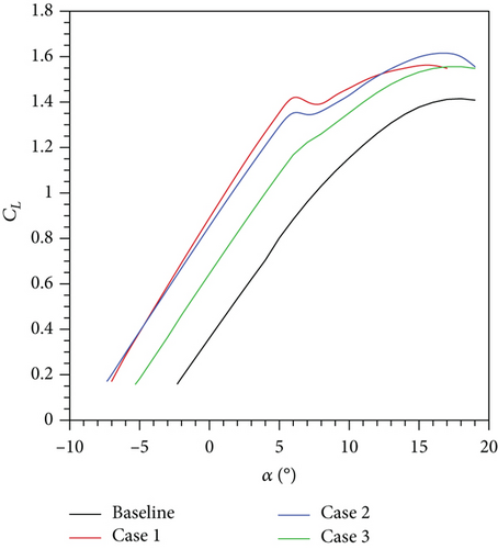
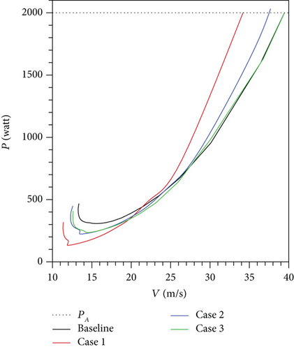
According to the results, the highest maximum is obtained for the first optimization problem when α₁ is 5.56° and V₁ is 11.97 m/s as depicted in Table 4. This corresponds to the neck in the C_L − α curve in Figure 11. Contrary to this, M_b at maximum nearly doubles and the increment in W_w is about 55%. According to the results in Figure 12, V_max of the first optimization problem is 34.2 m/s that is nearly 5 m/s less than the V_max of the baseline UAV. V_stall of the first optimization problem is 11.33 m/s that is almost the same as its V₁. The main reason for this situation is C_L of the maximum is very close to the maximum lift coefficient . When the airfoil shape and the wing planform details in Table 5 and Figures 13 and 14 are investigated, it is seen that the airfoil of the first optimization problem reaches the lower limit of the thickness and the upper limit of the camber. c_t and b are set to the lower limit and upper limit, respectively. c_r is decreased from 0.45 m to 0.386 m that alters the taper ratio (λ) from 1 to 0.52.

Table 4. Performance parameters of baseline UAV and the optimum UAVs.

	Baseline UAV	Case 1	Case 2	Case 3
	14.08	30.79	18.95	18.21
(°)	8	5.56	5.69	6.44
(m/s)	15.52	11.97	13.41	14.41
(Nm)	127.46	249.4	127.3	127.4
W_w (N)	24.06	37.64	19.41	21.8
V₂ (m/s)	39.45			39.45
α₂ at V₂ (°)	-2.32			-5.3
V₃ (m/s)	13.25			12.58
α₃ at V₃ (°)	18			17.86

Table 5. Geometric properties of the wings of the baseline UAV and the optimum UAV wings.

	Baseline UAV	Case 1	Case 2	Case 3
t	0.12	0.08	0.08	0.092
p	0.4	0.524	0.566	0.494
m	0.04	0.08	0.08	0.063
c_r (m)	0.45	0.386	0.586	0.596
c_t (m)	0.45	0.2	0.2	0.2
b (m)	4	8	4.578	4.524
S (m²)	1.8	2.34	1.8	1.8

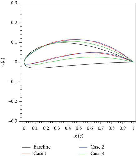
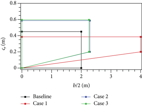
The airfoil shape of the second optimization problem is almost identical to the airfoil shape of the first optimization problem. Contrary to this, c_r and b have significant change due to the addition of the functional constraints related with M_b at the maximum and S. M_b reaches its upper limit whereas S is at its lower limit. But W_w is distant from its bound. As a result, the increment at the maximum is decreased from 220% to 34.6%. V_max of the second optimization problem is 37.2 m/s according to the P_R − V curve in Figure 12 whereas the V_stall is 12.3 m/s. Since S is decreased from 2.34 m² to 1.8 m², the increase in V_stall is observed.

The wing planform shape of the third optimization problem is almost the same as the wing planform shape of the second optimization problem. As clearly seen in the results, the functional constraints related with M_b at the maximum and S are the key reason for the similar outcomes from the different optimization problems. They reach their limits whenever they are defined as the functional constraints. V_max of the third optimization problem is identical to V₂ of the same problem according to Table 4 and Figure 12. This implies that the third optimization problem barely has the same V_max of the baseline UAV. The airfoil of the third optimization problem is thicker and less cambered when it is compared with the airfoil of the second optimization problem. This change is caused by the addition of the level flight performance analysis at the V₂ speed. V_stall of the third optimization problem is approximately 0.7 m/s less than V_stall of the baseline UAV. According to this result, it can be said that defining a functional constraint related with V_stall in maximization problems has no significant contribution, because all optimized wings satisfy the level flight condition at a speed less than V_stall of the baseline UAV.

Table 6 depicts the number of iterations (I), the number of the function count (fc), and the elapsed solution time (t_e) of the optimization problems. According to the result, the third optimization problem has the longest solution time because the aerodynamic design tool is called three times at each function count due to the analysis of three different level flight phases. t_e of the third problem is 6.64 hours. If ANSYS-Fluent was used as a function evaluator in the third optimization problem, t_e would be around 500 hours. This comparison shows the cost and time effectiveness of the aerodynamic analysis tool.

Table 6. I, fc, and t_e of Case 1, Case 2, and Case 3.

	Case 1	Case 2	Case 3
I	13	18	12
fc	32	26	38
t_e (s)	8520	10505	23896

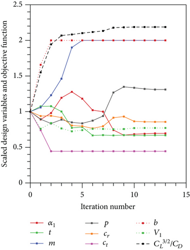
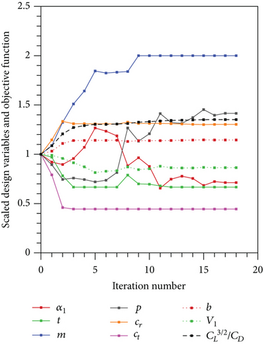
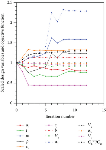
The evaluation of the design variables and the objective function with the iteration number for the optimization problems are presented in Figures 15, 16, and 17.

4. Conclusion

This paper demonstrates a rapid aerodynamic design tool for the wing optimization by using the maximum thickness, the maximum camber, the maximum camber location, the root chord, the tip chord, the span, the free stream velocity, and the angle of attack as the design variables. The function evaluator of the aerodynamic design tool consists of the Xfoil and nonlinear numerical lifting-line theory. Sequential quadratic programming is the optimization solver in the design tool. The derivatives of the objective function and the constraints with respect to the design variables are obtained by the use of parallel programming. Three different optimization problems are solved. According to the results,

(1)
Defining the functional constraint related to the stall speed performance of the UAV in maximization problems has no effect because all optimized UAVs have less stall speed than the baseline UAV. Moreover, the stall speed analysis increases the solution time
(2)
When the bending moment at the root, the wing weight, and the wing planform are limited at the same time, the bending moment reaches its upper limit whereas the wing area is at its lower limit. Contrary to this, the wing weight is distant from its upper limit. That means the bending moment at the root and the planform area constraints form the planform shape. But their effect on the airfoil shape change is insignificant
(3)
Limiting the maximum speed of the UAV yields thicker and less cambered airfoil

In summary, defining the constraints related to the bending moment at the root, the wing area, and the maximum speed of the UAV ensures the evaluation of the outcomes of the optimization problems to the more down-to-earth design results.

Conflicts of Interest

The authors declare that there is no conflict of interest regarding the publication of this paper.

Open Research

Data Availability

The data used to support the findings of this study are available from the corresponding author upon request.

References

1 Kroo I. M., Altus S., Braun R., Gage P., and Sobieski I., Multidisciplinary optimization methods for aircraft preliminary design, 5th AIAA/USAF/NASA/ISSMO Symposium on Multidisciplinary Analysis and Optimization, September 1994, Panama City Beach, FL, USA, https://doi.org/10.2514/6.1994-4325.
10.2514/6.1994-4325
Google Scholar
2 Drela M., "XFOIL: an analysis and design system for low Reynolds number airfoils." Low Reynolds number aerodynamics, 1989, Springer, Berlin, Heidelberg.
Google Scholar
3 Drela M. and Giles M. B., Viscous-inviscid analysis of transonic and low Reynolds number airfoils, AIAA Journal. (1987) 25, no. 10, 1347–1355, https://doi.org/10.2514/3.9789, 2-s2.0-0023437684.
10.2514/3.9789
Web of Science® Google Scholar
4 Koreanschi A., Oliviu S. G., Ayrault T., Botez R. M., Mamou M., and Mebarki Y., Numerical optimization and experimental testing of a morphing wing with aileron system, 24th AIAA/AHS Adaptive Structures Conference, January 2016, San Diego, CA, USA, https://doi.org/10.2514/6.2016-1083.
10.2514/6.2016-1083
Google Scholar
5 Gabor O. Ş., Simon A., Koreanschi A., and Botez R. M., Improving the UAS-S4 Éhecal airfoil high angles-of-attack performance characteristics using a morphing wing approach, Proceedings of the Institution of Mechanical Engineers, Part G: Journal of Aerospace Engineering. (2016) 230, no. 1, 118–131, https://doi.org/10.1177/0954410015587725, 2-s2.0-84951842793.
10.1177/0954410015587725
Web of Science® Google Scholar
6 Della Vecchia P., Corcione S., Pecora R., Nicolosi F., Dimino I., and Concilio A., Design and integration sensitivity of a morphing trailing edge on a reference airfoil: the effect on high-altitude long-endurance aircraft performance, Journal of Intelligent Material Systems and Structures. (2017) 28, no. 20, 2933–2946, https://doi.org/10.1177/1045389x17704521, 2-s2.0-85038072473.
10.1177/1045389X17704521
Web of Science® Google Scholar
7 Magrini A. and Benini E., Aerodynamic optimization of a morphing leading edge airfoil with a constant arc length parameterization, Journal of Aerospace Engineering. (2017) 31, no. 2, article 04017093, https://doi.org/10.1061/(ASCE)AS.1943-5525.0000812, 2-s2.0-85035312804.
10.1061/(ASCE)AS.1943-5525.0000812
Web of Science® Google Scholar
8 Liu Z., Dong L., Moschetta J. M., Zhao J., and Yan G., Optimization of nano-rotor blade airfoil using controlled elitist NSGA-II, International Journal of Micro Air Vehicles. (2014) 6, no. 1, 29–42, https://doi.org/10.1260/1756-8293.6.1.29, 2-s2.0-84897440834.
10.1260/1756-8293.6.1.29
Web of Science® Google Scholar
9 Silvestre M. A., Morgado J. P., and Pascoa J., JBLADE: a propeller design and analysis code, 2013 International Powered Lift Conference, August 2013, Los Angeles, CA, https://doi.org/10.2514/6.2013-4220, 2-s2.0-84883480749.
10.2514/6.2013-4220
Google Scholar
10 Anderson J. D. and Corda S., Numerical lifting line theory applied to drooped leading-edge wings below and above stall, Journal of Aircraft. (1980) 17, no. 12, 898–904, https://doi.org/10.2514/3.44690, 2-s2.0-0019265564.
10.2514/3.44690
Web of Science® Google Scholar
11 Gamboa P., Vale J., Lau F. J. P., and Suleman A., Optimization of a morphing wing based on coupled aerodynamic and structural constraints, AIAA Journal. (2009) 47, no. 9, 2087–2104, https://doi.org/10.2514/1.39016, 2-s2.0-73649084464.
10.2514/1.39016
Web of Science® Google Scholar
12 Merz C. B., Wolf C. C., Richter K., Kaufmann K., Mielke A., and Raffel M., Spanwise differences in static and dynamic stall on a pitching rotor blade tip model, Journal of the American Helicopter Society. (2017) 62, no. 1, 1–11, https://doi.org/10.4050/jahs.62.012002, 2-s2.0-85013272373.
10.4050/JAHS.62.012002
PubMed Web of Science® Google Scholar
13 AndersonJ. D.Jr., Fundamentals of aerodynamics, 2010, Tata McGraw-Hill Education.
Google Scholar
14 Lee J., Tan K. B., and Wang P. C., Parametric investigation of box wing configuration in viscous flow regime, 2018 Applied Aerodynamics Conference, June 2018, Atlanta, GA, US, https://doi.org/10.2514/6.2018-3814, 2-s2.0-85051723949.
10.2514/6.2018-3814
Google Scholar
15 https://web.mit.edu/drela/Public/web/xfoil/.
Google Scholar
16 https://www.mathworks.com/matlabcentral/fileexchange/30446-xfoil-interface.
Google Scholar
17 Pate D. J. and German B. J., Lift distributions for minimum induced drag with generalized bending moment constraints, Journal of Aircraft. (2013) 50, no. 3, 936–946, https://doi.org/10.2514/1.c032074, 2-s2.0-84880956136.
10.2514/1.C032074
Web of Science® Google Scholar
18 Sterligov B. and Cherkasov S., Reducing magnetic noise of an unmanned aerial vehicle for high-quality magnetic surveys, International Journal of Geophysics. (2016) 2016, 7, https://doi.org/10.1155/2016/4098275, 2-s2.0-84961901881.
10.1155/2016/4098275
Google Scholar
19 Hassanalian M., Throneberry G., Ali M., Ayed S. B., and Abdelkefi A., Role of wing color and seasonal changes in ambient temperature and solar irradiation on predicted flight efficiency of the albatross, Journal of Thermal Biology. (2018) 71, 112–122, https://doi.org/10.1016/j.jtherbio.2017.11.002, 2-s2.0-85035108498.
10.1016/j.jtherbio.2017.11.002
CAS PubMed Web of Science® Google Scholar
20 Communier D., Salinas M. F., Carranza Moyao O., and Botez R. M., Aero structural modeling of a wing using CATIA V5 and XFLR5 software and experimental validation using the Price-Païdoussis wing tunnel, AIAA Atmospheric Flight Mechanics Conference, June 2015, Dallas, TX.
Google Scholar
21 Langtry R. B. and Menter F. R., Correlation-based transition modeling for unstructured parallelized computational fluid dynamics codes, AIAA journal. (2009) 47, no. 12, 2894–2906, https://doi.org/10.2514/1.42362, 2-s2.0-73549112177.
10.2514/1.42362
Web of Science® Google Scholar
22 Aftab S. M. A., Rafie A. M., Razak N. A., and Ahmad K. A., Turbulence model selection for low Reynolds number flows, PloS one. (2016) 11, no. 4, article e0153755, https://doi.org/10.1371/journal.pone.0153755, 2-s2.0-84977647778.
10.1371/journal.pone.0153755
Web of Science® Google Scholar
23 Lanzafame R., Mauro S., and Messina M., Wind turbine CFD modeling using a correlation-based transitional model, Renewable Energy. (2013) 52, 31–39, https://doi.org/10.1016/j.renene.2012.10.007, 2-s2.0-84869112361.
10.1016/j.renene.2012.10.007
Web of Science® Google Scholar
24 ANSYS, Fluent Theory Guide, 2013.
Google Scholar
25 Thomas J. L. and Salas M. D., Far-field boundary conditions for transonic lifting solutions to the Euler equations, AIAA Journal. (1986) 24, no. 7, 1074–1080, https://doi.org/10.2514/3.9394, 2-s2.0-0022751897.
10.2514/3.9394
Web of Science® Google Scholar
26 Menter F. R., Langtry R. B., Likki S. R., Suzen Y. B., Huang P. G., and Völker S., A correlation-based transition model using local variables—part I: model formulation, Journal of Turbomachinery. (2006) 128, no. 3, 413–422, https://doi.org/10.1115/1.2184352, 2-s2.0-33845684578.
10.1115/1.2184352
Web of Science® Google Scholar
27 https://web.mit.edu/drela/Public/web/xfoil/xfoil6.99.tgz.
Google Scholar
28 Prytz E. R., Huuse Ø., Müller B., Bartl J., and Sætran L. R., Numerical simulation of flow around the NREL S826 airfoil at moderate Reynolds number using delayed detached Eddy simulation (DDES), AIP Conference Proceedings. (2017) 1863, no. 1, article 560086, AIP Publishinghttps://doi.org/10.1063/1.4992769, 2-s2.0-85026659730.
10.1063/1.4992769
Google Scholar
29 Vanderplaats G. N., Numerical optimization techniques for engineering design, 1984, 1999, 3rd edition, Vanderplaats R&D, Inc.
Google Scholar
30 Lasdon L. S. and Waren A. D., Large scale nonlinear programming, Computers & Chemical Engineering. (1983) 7, no. 5, 595–604, https://doi.org/10.1016/0098-1354(83)80005-2, 2-s2.0-0020221028.
10.1016/0098-1354(83)80005-2
Web of Science® Google Scholar
31 Sadraey M. H., Aircraft design: a systems engineering approach, 2012, John Wiley & Sons.
10.1002/9781118352700
Google Scholar
32 Sadraey M., Aircraft performance: analysis, 2009, VDM Publishing.
Google Scholar

Citing Literature

All articles

Aerodynamic Optimization of a UAV Wing subject to Weight, Geometric, Root Bending Moment, and Performance Constraints

Abstract

1. Introduction

2. Method

2.1. The Nonlinear Numerical Lifting-Line Theory

2.2. XFLR5 LLT and ANSYS-Fluent γ − Re_θ SST Model

2.3. Comparison of the Aerodynamic Analysis Tool with ANSYS-Fluent

2.4. Optimization Solver

2.5. The Characteristics of the Baseline UAV

3. Results

3.1. The Optimization Problems

3.2. Comparison of the Optimization Problem Solutions

4. Conclusion

Conflicts of Interest

Open Research

Data Availability

References

Citing Literature

Figures

References

Information

About Wiley Online Library

Help & Support

Opportunities

Connect with Wiley

Aerodynamic Optimization of a UAV Wing subject to Weight, Geometric, Root Bending Moment, and Performance Constraints

Abstract

1. Introduction

2. Method

2.1. The Nonlinear Numerical Lifting-Line Theory

2.2. XFLR5 LLT and ANSYS-Fluent γ − Reθ SST Model

2.3. Comparison of the Aerodynamic Analysis Tool with ANSYS-Fluent

2.4. Optimization Solver

2.5. The Characteristics of the Baseline UAV

3. Results

3.1. The Optimization Problems

3.2. Comparison of the Optimization Problem Solutions

4. Conclusion

Conflicts of Interest

Open Research

Data Availability

References

Citing Literature

Figures

References

Related

Information

2.2. XFLR5 LLT and ANSYS-Fluent γ − Re_θ SST Model