When the coarse-resolution observations used in the first step of multiscale and multistep variational data assimilation become increasingly nonuniform and/or sparse, the error variance of the first-step analysis tends to have increasingly large spatial variations. However, the analysis error variance computed from the previously developed spectral formulations is constant and thus limited to represent only the spatially averaged error variance. To overcome this limitation, analytic formulations are constructed to efficiently estimate the spatial variation of analysis error variance and associated spatial variation in analysis error covariance. First, a suite of formulations is constructed to efficiently estimate the error variance reduction produced by analyzing the coarse-resolution observations in one- and two-dimensional spaces with increased complexity and generality (from uniformly distributed observations with periodic extension to nonuniformly distributed observations without periodic extension). Then, three different formulations are constructed for using the estimated analysis error variance to modify the analysis error covariance computed from the spectral formulations. The successively improved accuracies of these three formulations and their increasingly positive impacts on the two-step variational analysis (or multistep variational analysis in first two steps) are demonstrated by idealized experiments.

1. Introduction

Multiple Gaussians with different decorrelation length scales have been used at NCEP to model the background error covariance in variational data assimilation (Wu et al. [1], Purser et al. [2]), but mesoscale features are still poorly resolved in the analyzed incremental fields even in areas covered by remotely sensed high-resolution observations, such as those from operational weather radars (Liu et al. [3]). This problem is common for the widely adopted single-step approach in operational variational data assimilation, especially when patchy high-resolution observations, such as those remotely sensed from radars and satellites, are assimilated together with coarse-resolution observations into a high-resolution model. To solve this problem, multiscale and multistep approaches were explored and proposed by several authors (Xie et al. [4], Gao et al. [5], Li et al. [6], and Xu et al. [7, 8]). For a two-step approach (or the first two steps of a multistep approach) in which broadly distributed coarse-resolution observations are analyzed first and then locally distributed high-resolution observations are analyzed in the second step, an important issue is how to objectively estimate or efficiently compute the analysis error covariance for the analyzed field that is obtained in the first step and used to update the background field in the second step. To address this issue, spectral formulations were derived by Xu et al. [8] for estimating the analysis error covariance. As shown in Xu et al. [8], the analysis error covariance can be computed very efficiently from the spectral formulations with very (or fairly) good approximations for uniformly (or nonuniformly) distributed coarse-resolution observations and, by using the approximately computed analysis error covariance, the two-step analysis can outperform the single-step analysis under the same computational constraint (that mimics the operational situation).

The analysis error covariance functions computed from the spectral formulations in Xu et al. [8] are spatially homogeneous, so their associated error variances are spatially constant. Although such a constant error variance can represent the spatial averaged value of the true analysis error variance, it cannot capture the spatial variation in the true analysis error variance. The true analysis error variance can have significant spatial variations, especially when the coarse-resolution observations become increasingly nonuniform and/or sparse. In this case, the spatial variation of analysis error variance and associated spatial variation in analysis error covariance need to be estimated based on the spatial distribution of the coarse-resolution observations in order to further improve the two-step analysis. This paper aims to explore and address this issue beyond the preliminary study reported in Xu and Wei [9]. In particular, as will be shown in this paper, analytic formulations for efficiently estimating the spatial variation of analysis error variance can be constructed by properly combining the error variance reduction produced by analyzing each and every coarse-resolution observation as a single observation, and the estimated analysis error variance can be used to further estimate the related variation in analysis error covariance. The detailed formulations are presented for one-dimensional cases first in the next section and then extended to two-dimensional cases in Section 3. Idealized numerical experiments are performed for one-dimensional cases in Section 4 and for two-dimensional cases in Section 5 to show the effectiveness of these formulations for improving the two-step analysis. Conclusions follow in Section 6.

2. Analysis Error Variance Formulations for One-Dimensional Cases

2.1. Error Variance Reduction Produced by a Single Observation

When observations are optimally analyzed in terms of the Bayesian estimation (see chapter 7 of Jazwinski [10]), the background state vector b is updated to the analysis state vector a with the following analysis increment:

(1a)

and the background error covariance matrix B is updated to the analysis error covariance matrix A according to

(1b)

where R is the observation error covariance matrix, d = y − h(b) is the innovation vector (observation minus background in the observation space), y is the observation vector, h() denotes the observation operator, and H is the linearized h(). For a single observation, say, at x_m in the one-dimensional space of x, the inverse matrix

reduces to

, so the ith diagonal element of A in (1b) is simply given by

(2)

where

(or

) is the background (or observation) error variance, C_b(x) is the background error correlation function, x_i denotes the ith point in the discretized analysis space R^N, and N is the number of grid points over the analysis domain. The length of the analysis domain is D = NΔx, where Δx is the analysis grid spacing and D is assumed to be much larger than the background error decorrelation length scale L.

Note that C_b(x) is a continuous function of x, so (2) can be written into

also as a continuous function of x, where

(3)

is the error variance reduction produced by analyzing a single observation at x = x_m. The error variance reduction in (3) decreases rapidly as |x − x_m| increases, and it becomes much smaller than it peak value of

at x = x_m as |x − x_m| increases to L. This implies that the error variance reduction produced by analyzing M sparsely distributed coarse-resolution observations can be estimated by properly combining the error variance reduction computed by (3) for each coarse-resolution observation as a single observation. This idea is explored in the following three subsections for one-dimensional cases with successively increased complexity and generality: from uniformly distributed coarse-resolution observations with periodic extension to nonuniformly distributed coarse-resolution observations without periodic extension.

2.2. Uniform Coarse-Resolution Observations with Periodic Extension

Consider that there are M coarse-resolution observations uniformly distributed in the above analysis domain of length D with periodic extension, so their resolution is Δx_co ≡ D/M. In this case, the error variance reduction produced by each observation can be considered as an additional reduction to the reduction produced by its neighboring observations, and this additional reduction is always smaller than the reduction produced by the same observation but treated as a single observation. This implies that the error variance reduction produced by analyzing the M coarse-resolution observations, denoted by

, is bounded above by

; that is,

(4)

where ∑_m denotes the summation over m for the M observations. The equality in (4) is for the limiting case of Δx_co/L → ∞ only. The inequality in (4) implies that the domain-averaged value of

is larger than the true averaged reduction estimated by

, where

is the domain-averaged analysis error variance estimated by the spectral formulation for one-dimensional cases in Section 2.2 of Xu et al. [8].

The domain-averaged value of

can be computed by

(5a)

where ∫_Ddx denotes the integration over the analysis domain, ∑_i denotes the summation over i for the N grid points, and D = NΔx is used in the last step. By extending

with the analysis domain periodically,

can be also estimated analytically as follows:

(5b)

where ∫dx denotes the integration over the infinite space of x,

is used in the second to last step, and

is used with Δx_co ≡ D/M in the last step. For the double-Gaussian form of C_b(x) = 0.6exp⁡(−x²/2L²) + 0.4exp⁡(−2x²/L²) used in (5) of Xu et al. [8], we have I₁ = (2π) ^1/2(0.44/2^1/2 + 0.48/5^1/2). The analytically derived value in (5b) is very close to (slightly larger than) the numerically computed value from (5a). With the domain-averaged value of

adjusted from

can be estimated by

(6)

The analysis error variance,

, is then estimated by

(7)

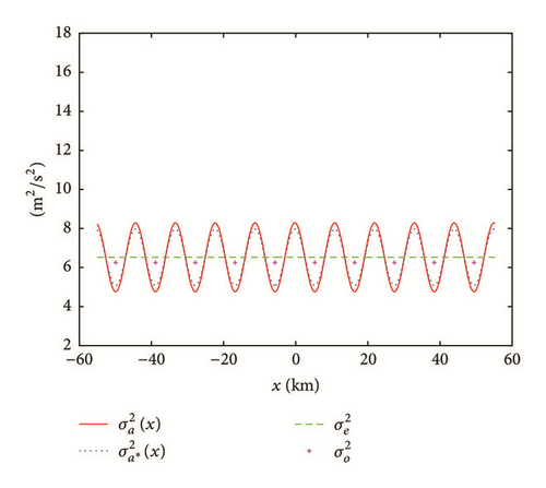
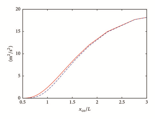
As shown by the example in Figure 1 (in which D = 110.4 km and M = 10 so Δx_co = D/M = 11.04 km is close to L = 10 km), the estimated in (7) has nearly the same spatial variation as the benchmark that is computed precisely from (1b), although the amplitude of spatial variation of , defined by , is slightly smaller than that of the true , defined by . As shown in Figure 2, the amplitude of spatial variation of benchmark decreases rapidly to virtually zero and then exactly zero (or increases monotonically toward its asymptotic upper limit of m² s⁻²) as Δx_co/L decreases to 0.5 and then to Δx/L = 0.1 (or increases toward ∞), and this decrease (or increase) of the amplitude of spatial variation of with Δx_co/L is closely captured by the amplitude of spatial variation of the estimated as a function of Δx_co/L.

Details are in the caption following the image — **Figure 1**
Open in figure viewer PowerPoint

Benchmark analysis error variance plotted by red solid curve and estimated analysis error variance in (7) plotted by blue dotted curve. The green dashed line shows the constant analysis error variance estimated from the spectral formulation. The purple + signs show the observation error variance ( m²s⁻²) at the locations of M (=10) uniformly distributed coarse-resolution observations with Δx_co = D/M (=11.04 km). The background error covariance has the double-Gaussian form with C_b(x) = 0.6 exp(−x²/2L²) + 0.4 exp(−2x²/L²), m²s⁻² and L = 10 km. The analysis domain length is D = NΔx = 110.4 km with N = 260 and Δx = 0.24 km, and the number of coarse-resolution observations is M = 10.

Using the estimated

in (7), the previously estimated analysis error covariance matrix, denoted by A_e with its ijth element

obtained from the spectral formulations, can be modified into A_a, A_b, or A_c with its ijth element given by

(8a)

(8b)

(8c)

The formulation in (8a) is conventional, as in (2.1) of Purser et al. [2] or originally (11) of Rutherford [11], in which the covariance is modified by applying

separately to each entry (indexed by i and j) of C_a(x_i − x_j) to retain the self-adjointness. The second equation in (8a) shows that the conventional approach can be viewed alternatively as A_eij plus a correction term, the last term in (8a). Ideally, the correction term should completely offset the deviation of A_eij from the true covariance, but the correction term in (8a) offsets only a part of the deviation.

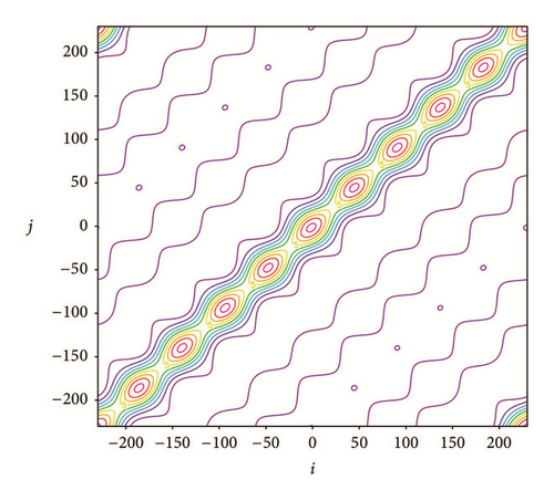
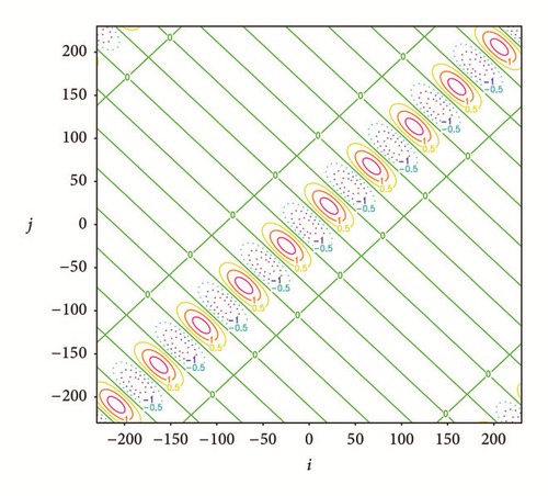
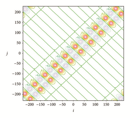
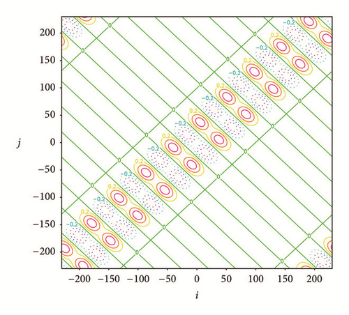
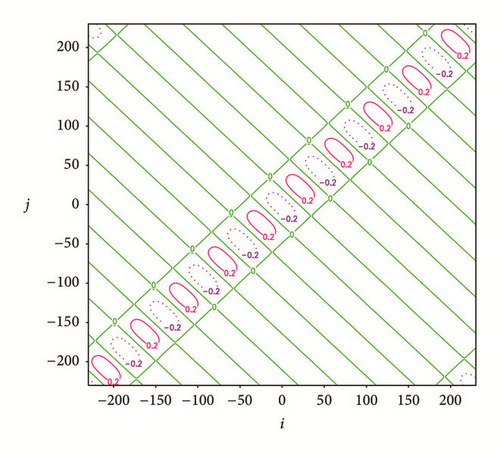
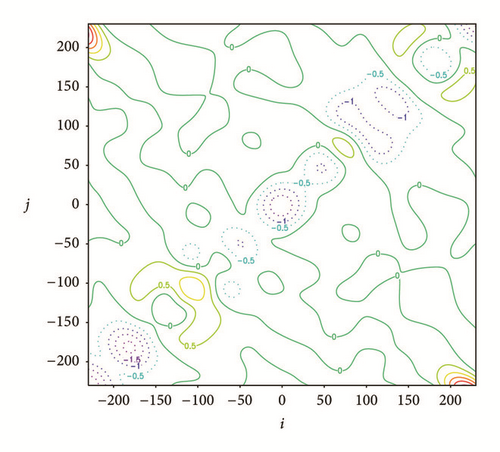
For the case in Figure 1, the benchmark analysis error covariance matrix, denoted by A, is computed precisely from (1b) and is plotted in Figure 3, while the deviations of A_e, A_a, A_b, and A_c from the benchmark A are shown in Figures 4(a), 4(b), 4(c), and 4(d), respectively. As shown, the deviation becomes increasingly small when A_e is modified successively to A_a, A_b, and A_c. Note that the correction term in (8a) is C_a(x_i − x_j) modulated by . This modulation has a chessboard structure, while the desired modulation revealed by the to-be-corrected deviation of A_c in Figure 4(a) has a banded structure (along the direction of x_i + x_j = constant, perpendicular to the diagonal line). This explains why the correction term in (8a) offsets only a part of the deviation as revealed by the deviation of A_a in Figure 4(b). On the other hand, the correction term in (8b) is modulated by . This modulation not only retains the self-adjointness but also has the desired banded structure, so the correction term in (8b) is an improvement over that in (8a), as shown by the deviation of A_b in Figure 4(c) versus that of A_a in Figure 4(b). However, as revealed by Figure 4(c), the deviation of A_b still has two significant maxima (or minima) along each band on the two sides of the diagonal line of x_i = x_j, while the to-be-corrected deviation of A_e in Figure 4(a) has a single maximum (or minimum) along each band. This implies that the function form of C_a(x_i − x_j) is not sufficiently wide for the correction. As a further improvement, this function form is widened to C_b(x_i − x_j) for the correction term in (8c), so the deviation of A_c in Figure 4(d) is further reduced from that of A_b in Figure 4(c).

When an estimated A is used to update the background error covariance in the second step for analyzing the high-resolution observations in the nested domain, the accuracy of the second-step analysis depends not only, to a certain extent, on the number of iterations performed by the minimization algorithm but also on the accuracy of the estimated A over the nested domain plus its extended vicinities within the distance of 2L_a outside the nested domain. Here, L_a is the decorrelation length scale of C_a(x) defined by

according to (4.3.10) of Daley [12], and L_a (=4.45 km for the case in Figures 1 and 3) can be easily computed as a by-product from the spectral formulation. Over this extended nested domain, the relative error (RE) of the estimated A_e with respect to the benchmark A can be measured by

(9)

where I_s denotes the unit matrix in the subspace associated with the grid points in the extended nested domain and thus I_s(A_e − A)I_s (or I_sAI_s) is the submatrix of A_e − A (or A) associated only with the grid points in the extended nested domain and ‖()‖_F denotes the Frobenius norm of () defined by the square root of the sum of the squared absolute values of the elements of the matrix in () according to (2.2–4) of Golub and Van Loan [13]. The REs of A_a, A_b, and A_c can be measured by the same form of Frobenius norm ratio as that defined for A_e in (9). The REs of A_e, A_a, A_b, and A_c are computed for the case in Figure 1 and listed in the first column of Table 1. As shown by the listed values, the RE becomes increasingly small when A_e is modified successively to A_a, A_b, and A_c, and this is consistent with and also quantifies the successively reduced deviation shown in Figures 4(a)–4(d).

Table 1. Entire-domain averaged RMS errors (in ms⁻¹) for the analysis increments obtained from SE, TEe, TEa, TEb, and TEc applied to the first set of innovations with periodic extension and consecutively increased n, where n is the number of iterations. All the RMS errors are evaluated with respect to the benchmark analysis increment. The relative error (RE) of the estimated analysis error covariance for updating the background error covariance in the second step of the two-step analysis is listed with the experiment name in the first column for each two-step experiment.

Experiment	n = 20	n = 50	n = 100	Final
SE	0.671	0.365	0.187	0.013 at n = 481
TEe with RE(A_e) = 0.229	0.171	0.150	0.142	0.135 at n = 210
TEa with RE(A_a) = 0.156	0.169	0.142	0.144	0.144 at n = 116
TEb with RE(A_b) = 0.101	0.147	0.098		0.090 at n = 67
TEc with RE(A_c) = 0.042	0.145	0.063	0.062	0.032 at n = 176

2.3. Nonuniform Coarse-Resolution Observations with Periodic Extension

Consider that the M coarse-resolution observations are now nonuniformly distributed in the analysis domain of length D with periodic extension, so their averaged resolution can be defined by Δx_co ≡ D/M. The spacing of a concerned coarse-resolution observation, say the mth observation, from its right (or left) adjacent observation can be denoted by Δx_com+ (or Δx_com−). Now we can consider the following two limiting cases.

First, we consider the case of Δx_com+ → 0 with Δx_com− = Δx_co (or Δx_com− → 0 with Δx_com+ = Δx_co). In this case, the concerned mth observation collapses onto the same point with its right (or left) adjacent observation, that is, the (m + 1)th [or (m − 1)th] observation. The two collapsed observations should be combined into one superobservation with a reduced error variance from

. The error variance reduction produced by this superobservation still can be estimated by (3) but with

(10a)

On the other hand, without super-Obbing, the error variance reduction produced by the two collapsed observations will be overestimated by (3) with

(10b)

By comparing (10b) with (10a), it is easy to see that this overestimation can be corrected if the error variance is inflated from

for each of the two collapsed observations.

Then, we consider the case of Δx_com+ → 0 and Δx_com− → 0. In this case, the concerned mth observation collapses with its two adjacent observations, that is, the (m + 1)th and (m − 1)th observations. The three collapsed observations should be combined into one superobservation with a reduced error variance from

. The error variance reduction produced by this superobservation still can be estimated by (3) but with

(10c)

On the other hand, without super-Obbing, the error variance reduction produced by the three collapsed observations will be overestimated by (3) with

(10d)

By comparing (10d) with (10c), it is easy to see that this overestimation can be corrected if the error variance is inflated from

for each of the three collapsed observations.

Based on the above analyses, when the error variance reduction produced by the mth observation is estimated by (3), the error variance should be adjusted for this observation unless Δx_com+ = Δx_com− = Δx_co. In particular, its error variance can be adjusted from

with β_m given empirically by

(11a)

Note that β_m = 2 for Δx_com+ = Δx_com− = 0, so the adjusted error variance is

which recovers the result derived from (10c)-(10d). Note also that β_m = 1 for Δx_com+ = 0 and Δx_com− = Δx_co (or Δx_com− = 0 and Δx_com+ = Δx_co), so the adjusted error variance is

which recovers the result derived from (10a)-(10b). Clearly, for Δx_com− = Δx_com+ = Δx_co, β_m = 0, so

is not adjusted which recovers the result for uniformly distributed coarse-resolution observations.

The above results suggest that

should be modified into

(11b)

This modification can improve the similarity of the spatial variation of

to that of the true error variance reduction, denoted by

, but the maximum (or minimum) of

, denoted by

(or

), is usually not very close to that of

. The maximum (or minimum) of

can be closely estimated by

(or

), the maximum (or minimum) of

computed by (6) for uniform coarse-resolution observations but with Δx_co decreased to Δx_omn (or increased to Δx_omx), where Δx_omn (or Δx_omx) is the minimum (or maximum) spacing between two adjacent observations among all nonuniformly distributed coarse-resolution observations in the one-dimension analysis domain. By adjusting

and

, the error variance reduction can be estimated by

(12a)

where

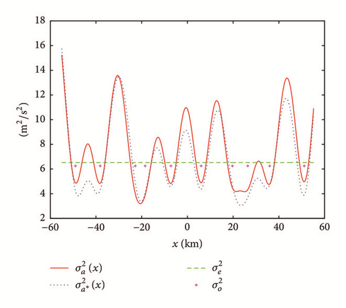
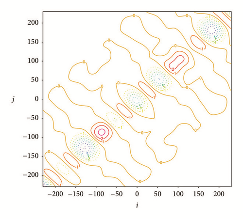
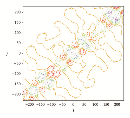
The analysis error variance is then estimated by as in (7), except that is computed by (12a) instead of (6). As shown by the example in Figure 5, the estimated captures closely not only the maximum and minimum but also the spatial variation of the benchmark computed from (1b). Using this estimated , the previously estimated A_e from the spectral formulation can be modified into A_a, A_b, or A_c with its ijth element given by the same formulation as shown in (8a), (8b), or (8c). For the case in Figure 5, the benchmark A is plotted in Figure 6, while the deviations of A_e, A_a, A_b, and A_c from the benchmark A are shown in Figures 7(a), 7(b), 7(c), and 7(d), respectively. As shown, the deviation becomes increasingly small when the estimated analysis error covariance matrix is modified successively to A_a, A_b, and A_c.

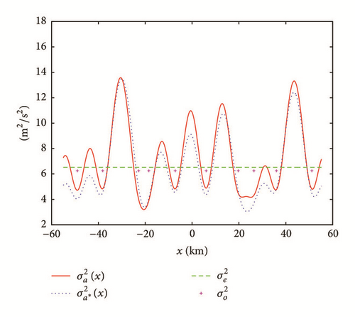
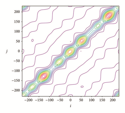
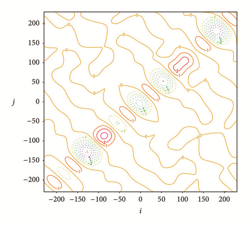
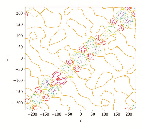
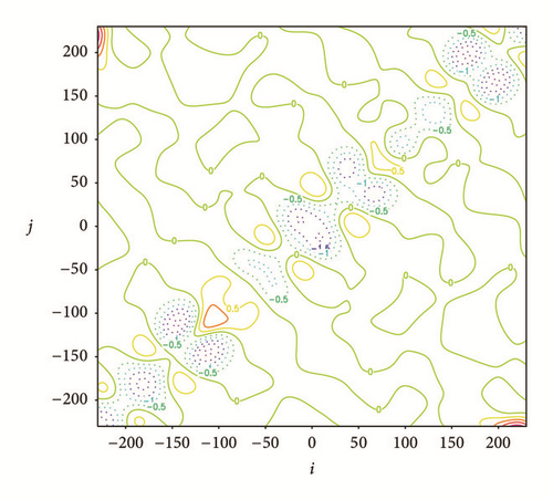
As explained in Section 2.2, the accuracy of the second-step analysis depends on the accuracy of the estimated A over the extended nested domain (i.e., the nested domain plus its extended vicinities within the distance of 2L_a on each side outside the nested domain), while the latter can be measured by the smallness of the RE of the estimated A with respect to the benchmark A, as defined for A_e in (9). The REs of A_e, A_a, A_b, and A_c computed for the case in Figure 5 are listed in the first column of Table 2. As listed, the RE becomes increasingly small when A_e is modified successively to A_a, A_b, and A_c, which quantifies the successively reduced deviation shown in Figures 7(a)–7(d).

Table 2. As in Table 1 but for the second set of innovations with periodic extension.

Experiment	n = 20	n = 50	n = 100	Final
SE	0.711	0.334	0.276	0.018 at n = 404
TEe with RE(A_e) = 0.355	0.482	0.439		0.442 at n = 76
TEa with RE(A_a) = 0.238	0.418	0.388	0.348	0.353 at n = 108
TEb with RE(A_b) = 0.197	0.318	0.288	0.257	0.243 at n = 179
TEc with RE(A_c) = 0.148	0.213	0.151		0.155 at n = 52

2.4. Nonuniform Coarse-Resolution Observations without Periodic Extension

Consider that the M coarse-resolution observations are still nonuniformly distributed in the one-dimensional analysis domain of length D but without periodic extension. In this case, their produced error variance reduction still can be estimated by (12a) except for the following three modifications.

(i) The maximum (or minimum) of , that is, (or ), should be found in the interior domain between the leftist and rightist observation points.

(ii) For the leftist (or rightist) observation that has only one adjacent observation to its right (or left) in the one-dimensional analysis domain, its error variance is still adjusted from to but β_m is calculated by setting [or (Δx_com+) = 0] in (11a) for calculating γ_m in (11b).

(iii) Note from (12a) that

and thus

as x moves outward far away from the leftist (or rightist) measurement point and thus far away from all the observations points. In this case, if

(as for the case in this section), then

estimated by F(x) in (12a) may become unrealistically negative as x moves outward beyond the leftist (or rightist) measurement point, denoted by x_mb. To avoid this problem, (12a) is modified into

(12b)

where R₁ is a factor defined by

(13)

It is easy to see from (12b) that for

and thus R₁ = 1,

as |x| → ∞, so the estimated

in (12b) can never become unrealistically negative.

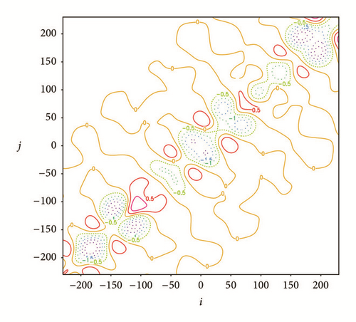
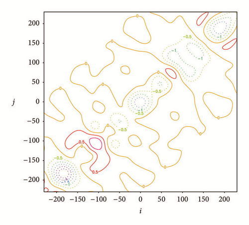
The analysis error variance is estimated by as in (7), except that is computed by (12a) [or (12b)] for x within (or beyond) the interior domain. As shown by the example in Figure 8, the estimated captures closely the spatial variation of the benchmark not only within but also beyond the interior domain. Using this estimated , A_e can be modified into A_a, A_b, or A_c with its ijth element given by the same formulation as shown in (8a), (8b), or (8c). For the case in Figure 8, the benchmark A (not shown) has the same interior structure (for interior grid points i and j) as that for the case with periodic extension in Figure 6, but significant differences are seen in the following two aspects around the four corners (similar to those seen from Figures 7(a) and 11(a) of Xu et al. [8]). (i) The element value becomes large toward the two corners along the diagonal line (which is consistent with the increased analysis error variance toward the two ends of the analysis domain as shown in Figure 8 in comparison with that in Figure 5). (ii) The element value becomes virtually zero toward the two off-diagonal corners (because there is no periodic extension). The deviations of A_e, A_a, A_b, and A_c from the benchmark A are shown in Figures 9(a), 9(b), 9(c), and 9(d), respectively, for the case in Figure 8. As shown, the deviation becomes increasingly small when the estimated analysis error covariance matrix is modified successively to A_a, A_b, and A_c. The REs of A_e, A_a, A_b, and A_c are listed in the first column of Table 3. As listed, the RE becomes increasingly small when A_e is modified successively to A_a, A_b, and A_c, which quantifies the successively reduced deviation shown in Figures 9(a)–9(d).

Table 3. As in Table 2 but for the third set of innovations without periodic extension.

Experiment	n = 20	n = 50	n = 100	Final
SE	0.499	0.328	0.194	0.012 at n = 451
TEe with RE(A_e) = 0.355	0.463	0.424		0.399 at n = 73
TEa with RE(A_a) = 0.238	0.394	0.358		0.385 at n = 54
TEb with RE(A_b) = 0.196	0.281	0.273		0.248 at n = 77
TEc with RE(A_c) = 0.147	0.215	0.149		0.123 at n = 77

3. Analysis Error Variance Formulations for Two-Dimensional Cases

3.1. Error Variance Reduction Produced by a Single Observation

For a single observation, say, at x_m ≡ (x_m, y_m) in the two-dimensional space of x = (x, y), the inverse matrix in (1b) also reduces to , so the ith diagonal element of A is given by the same formulation as in (2) except that x_i (or x_m) is replaced by x_i (or x_m). Here, x_i denotes the ith point in the discretized analysis space R^N with N = N_xN_y, N_x (or N_y) is the number of analysis grid points along the x (or y) direction in the two-dimensional analysis domain. The length (or width) of the analysis domain is D_x = N_xΔx (or D_y = N_yΔy) and is assumed to be much larger than the background error decorrelation length scale L in x, where Δx (or Δy) is the grid spacing in the x (or y) direction and Δx = Δy is assumed for simplicity.

Since C_b(x) is a continuous function of x, the aforementioned formulation for the ith diagonal element of A can be written into

also as a continuous function of x, where

(14)

is the error variance reduction produced by analyzing a single observation at x = x_m. This reduction decreases rapidly and becomes much smaller than it peak value of

at x = x_m as |x − x_m| increases to L and beyond.

3.2. Uniform Coarse-Resolution Observations with Periodic Extension

Consider that there are M coarse-resolution observations uniformly distributed in the above analysis domain of length D_x and width D_y with periodic extension along x and y, so their resolution is /M^1/2, where M = M_xM_y, M_x (or M_y) denotes the number of observations uniformly distributed along the x (or y) direction in the two-dimensional analysis domain, and D_x/M_x = D_y/M_y is assumed (so Δx_co = D_x/M_x = D_y/M_y). In this case, as explained for the one-dimensional case in Section 2.2, the error variance reduction produced by each observation can be considered as an additional reduction to the reduction produced by its neighboring observations. This additional reduction is smaller than the reduction produced by a single observation, so the error variance reduction produced by analyzing the M coarse-resolution observations is bounded above by , which is similar to that for the one-dimensional case in (4). For the same reason as explained for the one-dimensional case in (4), this implies that the domain-averaged value of is larger than the true averaged reduction estimated by , where is the domain-averaged analysis error variance estimated by the spectral formulation for two-dimensional cases in Section 2.3 of Xu et al. [8].

The domain-averaged value of

can be computed by

(15a)

where ∬_Ddx denotes the integration over the two-dimensional analysis domain, ∑_i denotes the summation over i for the N grid points, and D_xD_y = N_xΔxN_yΔy = NΔxΔy is used in the last step. By extending

with the analysis domain periodically in both the x and y directions,

can be estimated analytically as follows:

(15b)

where ∬dx = ∬dx dy denotes the integration over the entire space of x,

is used in the second to last step, and I₂ ≡ ∬dxC_b(x)/L² is used with

in the last step. For the double-Gaussian form of C_b(x) = 0.6exp⁡(−|x|²/2L²) + 0.4exp⁡(−2|x|²/L²) used in Section 4 of Xu et al. [8], we have I₂ = 2π(0.2 + 0.48/5). The derived value in (15b) is very close to the numerically computed value from (15a).

With the domain-averaged value adjusted from

can be estimated by the same formulation as in (6) except that x is replaced by x. The analysis error variance is then estimated by

(16)

As shown by the example in Figure 10, the estimated

in (16) is very close to the benchmark

computed precisely from (1b), and the deviation of

from the benchmark

is within (−0.21, 0.35) m²s⁻². On the other hand, the constant analysis error variance (

= 6.7 m²s⁻²) estimated by the spectral formulation deviates from the benchmark

widely from −1.91 to 2.22 m²s⁻².

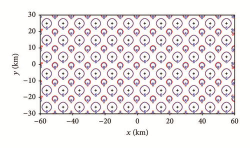
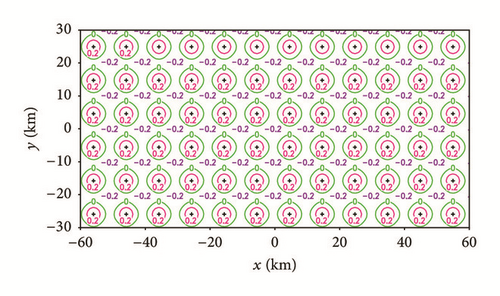
Using the estimated in (16), the previously estimated analysis error covariance matrix, denoted by A_e with its ijth element obtained from the spectral formulation, can be modified into A_a, A_b, or A_c with its ijth element given by the same formulation as in (8a), (8b), or (8c) except that x_i (or x_j) is replaced by x_i (or x_j). Again, as explained in Section 2.2 but for the two-dimensional case here, the accuracy of the second-step analysis depends on the accuracy of the estimated A over the extended nested domain, that is, the nested domain plus its extended vicinities within the distance of 2L_a outside the nested domain. Here, L_a is the decorrelation length scale of C_a(x) defined by according to (4.3.12) of Daley [12], and L_a (=4.52 km for the case in Figure 10) can be easily computed as a by-product from the spectral formulation. Over this extended nested domain, the relative error (RE) of each estimated A with respect to the benchmark A computed precisely from (1b) can be defined in the same way as that for A_e in (9), except that the extended nested domain is two-dimensional here. The REs of A_e, A_a, A_b, and A_c computed for the case in Figure 10 are listed in the first column of Table 4. As listed, the RE becomes increasingly small when A_e is modified successively to A_a, A_b, and A_c.

Table 4. As in Table 1 but for the two-dimensional case in Figure 10 in which the first set of two-dimensional innovations is used with periodic extension.

Experiment	n = 20	n = 50	n = 100	Final
SE	0.742	0.364	0.154	0.071 at n = 201
TEe with RE(A_e) = 0.233	0.394	0.185	0.108	0.104 at n = 140
TEa with RE(A_a) = 0.181	0.397	0.186	0.102	0.097 at n = 145
TEb with RE(A_b) = 0.130	0.403	0.183	0.089	0.085 at n = 133
TEc with RE(A_c) = 0.038	0.397	0.160	0.064	0.059 at n = 183

3.3. Nonuniform Coarse-Resolution Observations with Periodic Extension

Consider that the M coarse-resolution observations are now nonuniformly distributed in the analysis domain of length D_x and width D_y with periodic extension, so their averaged resolution can be defined by

. The spacing of a concerned coarse-resolution observation, say the mth observation, from its kth adjacent observation (among the total 4 adjacent observations), can be denoted by Δx_comk. Now we can consider the limiting case of Δx_comk → 0 for K (≤4) adjacent observations with Δx_comk = Δx_co for the remaining 4 − K (≥0) adjacent observations. In this case, the concerned mth observation collapses onto the same point with its K adjacent observations. The K + 1 collapsed observations should be combined into one superobservation with a reduced error variance from

. The error variance reduction produced by this superobservation still can be estimated by (14) but with

(17a)

On the other hand, without super-Obbing, the error variance reduction produced by the K + 1 collapsed observations will be overestimated by (14) with

(17b)

By comparing (17b) with (17a), it is easy to see that this overestimation can be corrected if the error variance is inflated from

for each of the (K + 1) collapsed observations.

Based on the above analyses, when the error variance reduction produced by the concerned mth observation is estimated by (14), the error variance should be adjusted for this observation unless Δx_comk = Δx_co for k = 1,2, 3, and 4. In particular,

can be adjusted to

with β_m given empirically by

(18a)

where

denotes the summation over k for the four adjacent observations nearest to the concerned mth observation. With β_m given by (18a), the adjusted

recovers not only the inflated observation error variance derived above for each limiting case [with Δx_cok → 0 for k = 1,2, …, K (≤4) and Δx_cok = Δx_co for the remaining 4 − K (≥0) observations] but also the original observation error variance

for uniformly distributed coarse-resolution observations.

The above results suggest that

should be modified into

(18b)

This modification can improve the similarity of the spatial variation of

to that of the true error variance reduction, denoted by

, but the maximum (or minimum) of

, denoted by

(or

), is usually not very close to that of

. The maximum (or minimum) of

can be estimated by

(or

), the maximum (or minimum) of

computed for uniformly distributed observations but with Δx_co decreased to Δx_omn (or increased to Δx_omx), where Δx_omn (or Δx_omx) is the minimum (or maximum) spacing of adjacent observations among all nonuniformly distributed coarse-resolution observations in the two-dimension analysis domain. Specifically, Δx_omn (or Δx_omx) is estimated by

with K = 2 and Δx_omx is estimated by

with K = 4, where x_m denotes the mth observation point, x_mk denotes the observation point that is kth nearest to x_m, min_m (or max_m) denotes the minimum (or maximum) over index m for all the coarse-resolution observation points in the two-dimension analysis domain,

denotes the summation over k from 1 to K, and K is the total number of adjacent observation points (nearest to x_m) used for estimating Δx_omn (with K = 2) or Δx_omx (or K = 4). By adjusting

and

, the error variance reduction can be estimated by

(19a)

where

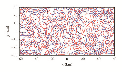
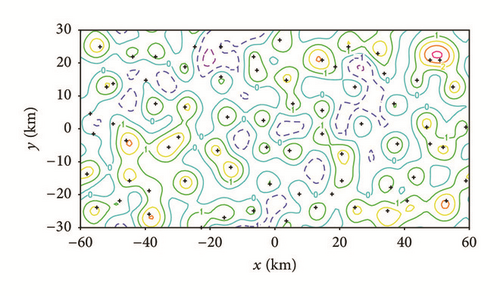
The analysis error variance is then estimated by as in (16), except that is computed by (19a). As shown by the example in Figure 11, the estimated (x) is fairly close to the benchmark , and the deviation of from the benchmark (x) is within (−2.40, 4.20) m²s⁻². On the other hand, the constant analysis error variance ( m²s⁻²) estimated by the spectral formulation deviates from the benchmark widely from −9.98 to 3.83 m²s⁻². Using this estimated , the previously estimated A_e from the spectral formulation can be modified into A_a, A_b, or A_c with its ijth element given by the same two-dimensional version of (8a), (8b), or (8c) as explained in Section 3.2. The REs of A_e, A_a, A_b, and A_c computed for the case in Figure 11 are listed in the first column of Table 5. As listed, the RE becomes increasingly small when A_e is modified successively to A_a, A_b, and A_c.

Table 5. As in Table 4 but for the two-dimensional case in Figure 11 where the second set of innovations is used with periodic extension.

Experiment	n = 20	n = 50	n = 100	Final
SE	0.757	0.364	0.175	0.069 at n = 241
TEe with RE(A_e) = 0.462	0.416	0.202	0.149	0.144 at n = 140
TEa with RE(A_a) = 0.274	0.411	0.202	0.143	0.144 at n = 215
TEb with RE(A_b) = 0.244	0.402	0.195	0.136	0.132 at n = 191
TEc with RE(A_c) = 0.165	0.403	0.179	0.106	0.103 at n = 287

3.4. Nonuniform Coarse-Resolution Observations without Periodic Extension

Consider that the M coarse-resolution observations are still nonuniformly distributed in the analysis domain of length D_x and width D_y but without periodic extension. In this case, their averaged resolution is still defined by . To estimate their produced error variance reduction, we need to modify the formulations constructed in the previous subsection with the following preparations. First, we need to identify four near-corner observations among all the coarse-resolution observations. Each near-corner observation is defined as the one that nearest to one of the four corners of the analysis domain. Then, we need to identify M_x − 2 (or M_y − 2) near-boundary observations associated with each x-boundary (or y-boundary), where M_x (or M_y) is estimated by the nearest integer to D_x/Δx_co (or D_y/Δx_co). The total number of near-boundary observations is thus given by 2(M_x + M_y) − 8. To identify these near-boundary observations, we need to divide the 2D domain uniformly along the x-direction and y-direction into M_xM_y boxes, so there are 2(M_x + M_y) − 8 boundary boxes (not including the four corner boxes). If a boundary box contains no coarse-resolution observation, then it is an empty box and should be substituted by its adjacent interior box (as a substituted boundary box). From each nonempty boundary box (including substituted boundary box), we can find one near-boundary observation that is nearest to the associated boundary. A closed loop of observation boundary can be constructed by piece-wise linear segments with every two neighboring near-boundary observation points connected by a linear segment and with each near-corner observation point connected by a linear segment to each of its two neighboring near-boundary observation points.

After the above preparations, the error variance reduction can be estimated by (19a) with the following three modifications:

(i) The maximum (or minimum) of , that is, (or ) should be found in the interior domain of |x | < D_x/2 − Δx_co and |y | < D_y/2 − Δx_co.

(ii) For each above defined near-boundary (or near-corner) observation that has only three (or two) adjacent observations, its error variance is still adjusted from to but β_m is calculated by setting in (18a) for k = 4 (or k = 3 and 4).

(iii) Note from (19a) that

and thus

as x moves outward far away from all the observations points. In this case, if

(as for the case in this section), then

estimated by (19a) may become unrealistically negative as x moves outward beyond the above constructed observation boundary loop. To avoid this problem, (19a) is modified into

(19b)

where R₂ is a factor defined by

(20)

x_mb is the projection of x on the observation boundary loop and the projection from x is along the direction normal to the x-associated domain boundary (nearest to x). However, if x is closer to a corner observation point than the remaining part of the observation boundary loop, then x_mb is simply that near-corner observation point. It is easy to see from (19b) that, for

and thus R₂ = 1,

as |x | →−∞, so the estimated

in (19b) can never become unrealistically negative.

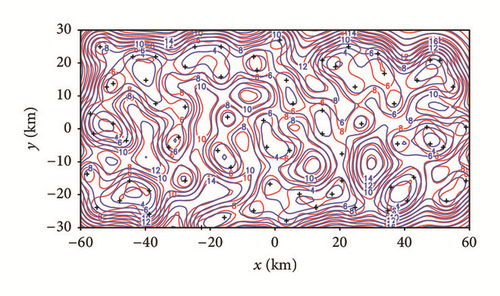
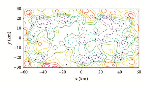
The analysis error variance is estimated by as in (16), except that is computed by (19a) [or (19b)] for x inside (or outside) the closed observation boundary loop. As shown by the example in Figure 12, the estimated is fairly close to the benchmark , and the deviation of from the benchmark is within (−4.08, 5.54) m²s⁻². On the other hand, the constant analysis error variance ( m²s⁻²) estimated by the spectral formulation deviates from the benchmark very widely from −16.1 to 3.82 m²s⁻². Using the estimated , the previously estimated A_e from the spectral formulation can be modified into A_a, A_b, or A_c with its ijth element given by the same two-dimensional version of (8a), (8b), or (8c) as explained in Section 3.2. The REs of A_e, A_a, A_b, and A_c computed for the case in Figure 12 are listed in the first column of Table 6. As listed, the RE becomes increasingly small when A_e is modified successively to A_a, A_b, and A_c.

Table 6. As in Table 5 but for the two-dimensional case in Figure 12 where the third set of innovations is used without periodic extension.

Experiment	n = 20	n = 50	n = 100	Final
SE	0.808	0.453	0.176	0.078 at n = 235
TEe with RE(A_e) = 0.462	0.509	0.179	0.136	0.134 at n = 161
TEa with RE(A_a) = 0.305	0.497	0.184	0.146	0.140 at n = 213
TEb with RE(A_b) = 0.258	0.495	0.179	0.135	0.127 at n = 170
TEc with RE(A_c) = 0.240	0.473	0.157	0.103	0.101 at n = 201

4. Numerical Experiments for One-Dimensional Cases

4.1. Experiment Design and Innovation Data

In this section, idealized one-dimensional experiments are designed and performed to examine to what extent the successively improved estimate of A in (8a), (8b), and (8c) can improve the two-step analysis. In particular, four types of two-step experiments, named TEe, TEa, TEb, and TEc, are designed for analyzing the high-resolution innovations in the second step with the background error covariance updated by A_e, A_a, A_b, and A_c, respectively, after the coarse-resolution innovations are analyzed in the first step. The TEe is similar to the first type of two-step experiment (named TEA) in Xu et al. [8], but the TEa, TEb, and TEc are new here. As in Xu et al. [8], a single-step experiment, named SE, is also designed for analyzing all the innovations in a single step. In each of the above five types of experiments, the analysis increment is obtained by using the standard conjugate gradient descent algorithm to minimize the cost-function (formulated as in (7) of Xu et al. [8]) with the number of iterations limited to n = 20, 50, or 100 before the final convergence to mimic the computationally constrained situations in operational data assimilation. Three sets of simulated innovations are generated for the above five types of experiments. The first set consists of M (=10) uniformly distributed coarse-resolution innovations over the analysis domain (see Figure 1) with periodic extension and M^′ (=74) high-resolution innovations in the nested domain of length D/6 (similar to those shown by the purple × signs in Figure 1 of Xu et al. [8] but generated at the grid points not covered by the coarse-resolution innovations within the nested domain). The second (or third) set is the same as the first set except that the coarse-resolution innovations are nonuniformly distributed with (or without) periodic extension as shown in Figure 5 (or Figure 8). All the innovations are generated by simulated observation errors subtracting simulated background errors at observation locations. Observation errors are sampled from computer-generated uncorrelated Gaussian random numbers with σ_o = 2.5 ms⁻¹ for both coarse-resolution and high-resolution observations. Background errors are sampled from computer-generated spatially correlated Gaussian random fields with σ_b = 5 ms⁻¹ and C_b(x) modeled by the double-Gaussian form given in Section 2.2 (also see the caption of Figure 1). The coarse-resolution innovations in the first, second, and third sets are thus generated in consistency with the three cases in Figures 1, 5, and 8, respectively.

4.2. Results from the First Set of Innovations

The first set of innovations is used here to perform each of the five types of experiments with the number of iterations limited to n = 20, 50, or 100 before the final convergence. The accuracy of the analysis increment obtained from each experiment with each limited n is measured by its domain-averaged RMS error (called RMS error for short hereafter) with respect to the benchmark analysis increment computed precisely from (1a). Table 1 lists the RMS errors of the analysis increments obtained from the SE, TEe, TEa, TEb, and TEc with the number of iterations increased from n = 20 to 50, 100, and/or the final convergence.

As shown in Table 1, the TEe outperforms SE for n = 20, 50, and 100 but not for n increased to the final convergence. The improved performance of TEe over SE is similar to but less significant than that of TEA over SE in Table 1 of Xu et al. [8]. The reduced improvement can be largely explained by the fact that the coarse-resolution innovations are generated here more sparsely and the deviation of A_e from the benchmark A is thus increased (as seen from Figure 4(a) in comparison with Figure 5(b) of Xu et al. [8]). The TEa outperforms TEe for n = 20 and 50 before n increased to 100 (which is very close to the final convergence at n = 116 for TEa). The improvement of TEa over TEe is consistent with and can be largely explained by the improved accuracy of A_a [RE(A_a) = 0.156] over A_e [RE(A_e) = 0.229]. The TEb outperforms TEa for n = 20 and 50 (before the final convergence at n = 67). The improvement of TEb over TEa is consistent with the improved accuracy of A_b [RE(A_b) = 0.101] over A_a. The TEc outperforms TEb for each listed value of n, and the improvement is consistent with the improved accuracy of A_c [with RE(A_c) = 0.042] over A_b.

4.3. Results from the Second Set of Innovations

The second set of innovations is used here to perform each of the five types of experiments with the number of iterations limited to n = 20, 50, or 100 before the final convergence. The domain-averaged RMS errors of the analysis increments obtained from the four two-step experiments are shown in Table 2 versus those from the SE. As shown, the TEe outperforms SE for n = 20 but not so for n = 50. The improvement of TEe over SE is similar to but much less significant than that of TEA over SE in Table 2 of Xu et al. [8]. This reduced improvement can be largely explained by the fact that the coarse-resolution innovations are generated here not only more sparsely but also more nonuniformly than those in Section 3.3 of Xu et al. [8] and the deviation of A_e from the benchmark A becomes much larger in Figure 7(a) here than that in Figure 7(b) of Xu et al. [8]. The TEa outperforms TEe for n = 20 and 50 but still underperforms SE for n increased to 50 and beyond. The improvement of TEa over TEe is consistent with the improved accuracy of A_a [RE(A_a) = 0.238] over A_e [RE(A_e) = 0.355]. The TEb outperforms TEa for each listed value of n and also outperforms SE for n up to 100. The improvement of TEb over TEa is consistent with the improved accuracy of A_b [RE(A_b) = 0.197] over A_a. The TEc outperforms TEb for each listed value of n, and the improvement is consistent with the improved accuracy of A_c [RE(A_c) = 0.148] over A_b.

4.4. Results from the Third Set of Innovations

The third set of innovations is used here to perform each of the five types of experiments with the number of iterations limited to n = 20, 50, or 100 before the final convergence. The domain-averaged RMS errors of the analysis increments obtained from the four two-step experiments are shown in Table 3 versus those from the SE. As shown, the TEe outperforms SE for n = 20 but not so for n = 50. The improvement of TEe over SE is much less significant than that of TEA over SE in Table 3 of Xu et al. [8], and this reduced improvement can be explained by the same fact as stated for the previous case in Section 4.3. The TEa outperforms TEe for n = 20 and 50, and the improvement is consistent with the improved accuracy of A_a [RE(A_a) = 0.238] over A_e [RE(A_e) = 0.355]. The TEb outperforms TEa for each listed value of n, which is consistent with the improved accuracy of A_b [RE(A_b) = 0.196] over A_a. The TEc outperforms TEb for each listed value of n, which is consistent with the improved accuracy of A_c [RE(A_c) = 0.147] over A_b.

5. Numerical Experiments for Two-Dimensional Cases

5.1. Experiment Design and Innovation Data

In this section, idealized two-dimensional experiments are designed and named similarly to those in Section 4 except that simulated innovations are generated in three sets for the two-dimensional cases in Figures 10, 11, and 12, respectively. In particular, the first set consists of M (= M_xM_y = 12 × 6) uniformly distributed coarse-resolution innovations over the periodic analysis domain (as shown in Figure 10) and M^′ (=66) high-resolution innovations generated at the grid points not covered by the coarse-resolution innovations within the nested domain. The nested domain (D_x/6 = 20 km long and D_y/6 = 10 km wide) is the same as that shown in Figure 16 of Xu et al. [8]. Again, all the innovations are generated by simulated observation errors subtracting simulated background errors at observation locations. Observation errors are sampled from computer-generated uncorrelated Gaussian random numbers with σ_o = 2.5 ms⁻¹ for both coarse-resolution and high-resolution observations. Background errors are sampled from computer-generated spatially correlated Gaussian random fields with σ_b = 5 ms⁻¹ and C_b(x) modeled by the double-Gaussian form given in Section 3.2 (also see the caption of Figure 10). The second (or third) set is the same as the first set except that the coarse-resolution innovations are nonuniformly distributed with (or without) periodic extension as shown in Figure 11 (or Figure 12).

5.2. Results from the First Set of Innovations

The first set of innovations is used here to perform each of the five types of experiments with the number of iterations limited to n = 20, 50, or 100 before the final convergence. The domain-averaged RMS errors of the analysis increments obtained from the four two-step experiments are shown in Table 4 versus those from the SE. As shown, the TEe outperforms SE for each listed value of n before the final convergence, which is similar to the improved performance of TEA over SE shown in Table 4 of Xu et al. [8]. The TEa outperforms TEe as n increases to 100 and beyond, which is consistent with the improved accuracy of A_a [RE(A_a) = 0.181] over A_e [RE(A_e) = 0.233]. The TEb outperforms TEa as n increases to 50 and beyond, which is consistent with the improved accuracy of A_b [RE(A_b) = 0.130] over A_a. The TEc outperforms TEb for each listed value of n, which is consistent with the improved accuracy of A_c [RE(A_c) = 0.038] over A_b.

5.3. Results from the Second Set of Innovations

5.4. Results from the Third Set of Innovations

The third set of innovations is used here to perform each of the five types of experiments with the number of iterations limited to n = 20, 50, or 100 before the final convergence. The domain-averaged RMS errors of the analysis increments obtained from the four two-step experiments are shown in Table 6 versus those from the SE. As shown, the TEe outperforms SE for each listed value of n before the final convergence. The improved performance of TEe over SE is similar to but less significant than that of TEA over SE in Table 5 of Xu et al. [8], and the reason is mainly because the coarse-resolution innovations are generated more sparsely and nonuniformly than those in Section 4.3 of Xu et al. [8]. The TEa outperforms TEe for n = 20 but not so as n increases to 50 and beyond, although A_a has an improved accuracy [RE(A_a) = 0.305] over A_e [RE(A_e) = 0.462]. The TEb outperforms TEa for each listed value of n, and the improved performance is consistent with the improved accuracy of A_b [RE(A_b) = 0.258] over A_a. The TEc outperforms TEb for each listed value of n, which is consistent with the improved accuracy of A_c [RE(A_c) = 0.240] over A_b.

6. Conclusions

In this paper, the two-step variational method developed in Xu et al. [8] for analyzing observations of different spatial resolutions is improved by considering and efficiently estimating the spatial variation of analysis error variance produced by analyzing coarse-resolution observations in the first step. The constant analysis error variance computed from the spectral formulations in Xu et al. [8] can represent the spatial averaged value of the true analysis error variance but it cannot capture the spatial variation in the true analysis error variance. As revealed by the examples presented in this paper (see Figures 1, 2, 5, and 8 for one-dimensional cases and Figures 10–12 for two-dimensional cases), the true analysis error variance tends to have increasingly large spatial variations when the coarse-resolution observations become increasingly nonuniform and/or sparse, and this is especially true and serious when the separation distances between neighboring coarse-resolution observations become close to or even locally larger than the background error decorrelation length scale. In this case, the spatial variation of analysis error variance and associated spatial variation in analysis error covariance need to be considered and estimated efficiently in order to further improve the two-step analysis.

The analysis error variance can be viewed equivalently and conveniently as the background error variance minus the total error variance reduction produced by analyzing all the coarse-resolution observations. To efficiently estimate the latter, analytic formulations are constructed for three types of coarse-resolution observations in one- and two-dimensional spaces with successively increased complexity and generality. The main results and major findings are summarized below for each type of coarse-resolution observations:

(i) The first type consists of uniformly distributed coarse-resolution observations with periodic extension. For this simplest type, the total error variance reduction is estimated in two steps. First, the error variance reduction produced by analyzing each coarse-resolution observation as a single observation is equally weighted and combined into the total. Then, the combined total error variance reduction is adjusted by a constant to match to the domain-averaged total error variance reduction estimated by the spectral formulation [see (5a), (5b), (15a), and (15b)]. The estimated analysis error variance (i.e., the background error variance minus the adjusted total error variance reduction) captures not only the domain-averaged value but also the spatial variation of the benchmark truth (see Figures 1, 2, and 10).

(ii) The second type consists of nonuniformly distributed coarse-resolution observations with periodic extension. For this more general type, the total error variance reduction is also estimated in two steps: The first step is similar to that for the first type but the combination into the total is weighted based on the averaged spacing of each concerned observation from its neighboring observations [see (11a), (11b), (18a), and (18b)]. In the second step, the combined total error variance reduction is adjusted and scaled to match the maximum and minimum of the true total error variance reduction estimated from the spectral formulation for uniformly distributed coarse-resolution observations but with the observation resolutions set, respectively, to the minimum spacing and maximum spacing of the nonuniformly distributed coarse-resolution observations [see (12a) and (19a)]. The estimated analysis error variance captures not only the maximum and minimum but also the spatial variation of the benchmark truth (see Figures 5 and 11).

(iii) The third type consists of nonuniformly distributed coarse-resolution observations without periodic extension. For this most general type, the total error variance reduction is estimated with the same two steps as for the second type, except that three modifications are made to improve the estimation near and at the domain boundaries [see (i)–(iii) in Sections 2.4 and 3.4]. The analysis error variance finally estimated captures the spatial variation of the benchmark truth not only in the interior domain but also near and at the domain boundaries (see Figures 8 and 12).

The above estimated spatially varying analysis error variance is used to modify the analysis error covariance computed from the spectral formulations of Xu et al. [8] in three different forms [see (8a), (8b), and (8c)]. The first is a conventional formulation in which the covariance is modulated by the spatially varying standard deviation separately via each entry of the covariance to retain the self-adjointness. This modulation has a chessboard structure but the desired modulation has a banded structure (along the direction perpendicular to the diagonal line) as revealed by the to-be-corrected deviation from the benchmark truth (see Figure 4(a)), so the deviation is only partially reduced (see Figure 4(b)). The second formulation is new, in which the modulation is realigned to capture the desired banded structure and yet still retain the self-adjointness. The deviation from the benchmark truth is thus further reduced (see Figure 4(c)), but the deviation is reduced not broadly enough along each band. By properly broadening the reduction distribution in the third formulation, the deviation is much further reduced (see Figure 4(d)).

The successive improvements made by the above three formulations are demonstrated for all the three types of coarse-resolution observations in one- and two-dimensional spaces. The improvements are quantified by the successively reduced relative errors [REs, measured by the Frobenius norm defined in (9)] of their modified analysis error covariance matrices with respect to the benchmark truths (see REs listed in the first columns of Tables 1–6). The impacts of the improved accuracies of the modified analysis error covariance matrices on the two-step analyses are examined with idealized experiments that are similar to but extend those in Xu et al. [8]. As expected, the impacts are found to be mostly positive (especially for the third formulation) and largely in consistency with the improved accuracies of the modified analysis error covariance matrices (see Tables 1–6). As new improvements to the conventional formulation, the second and third formulations may also be useful in constructing covariance matrices with nonconstant variances for general applications beyond this paper.

The formulations constructed in this paper for estimating the spatial variation of analysis error variance and associated spatial variation in analysis error covariance are effective for further improving the two-step variational method developed in Xu et al. [8], especially when the coarse-resolution observations become increasingly nonuniform and/or sparse. These formulations will be extended together with the spectral formulations of Xu et al. [8] for real-data applications in three-dimensional space with the variational data assimilation system of Gao et al. [5], in which the analyses are univariate and performed in two steps. Such an extension is currently being developed.

Conflicts of Interest

The authors declare that there are no conflicts of interest regarding the publication of this paper.

Acknowledgments

The authors are thankful to Dr. Jindong Gao for their constructive comments and suggestions that improved the presentation of the paper. The research work was supported by the ONR Grants N000141410281 and N000141712375 to the University of Oklahoma (OU). Funding was also provided to CIMMS by NOAA/Office of Oceanic and Atmospheric Research under NOAA-OU Cooperative Agreement no. NA11OAR4320072, US Department of Commerce.

References

1 Wu W.-S., Purser R. J., and Parrish D. F., Three-dimensional variational analysis with spatially inhomogeneous covariances, Monthly Weather Review. (2002) 130, no. 12, 2905–2916, 2-s2.0-0036968196, https://doi.org/10.1175/1520-0493(2002)130<2905:TDVAWS>2.0.CO;2.
10.1175/1520-0493(2002)130<2905:TDVAWS>2.0.CO;2
Web of Science® Google Scholar
2 Purser R. J., Wu W.-S., Parrish D. F., and Roberts N. M., Numerical aspects of the application of recursive filters to variational statistical analysis. Part II: Spatially inhomogeneous and anisotropic general covariances, Monthly Weather Review. (2003) 131, no. 8, 1536–1548, 2-s2.0-0141682980, https://doi.org/10.1175//2543.1.
10.1175//2543.1
Web of Science® Google Scholar
3 Liu S., Xue M., Gao J., and Parrish D., Analysis and impact of super-obbed Doppler radial velocity in the NCEP grid-point statistical interpolation (GSI) analysis system, Proceedings of the 21st Conference on on Weather Analysis and Forecasting/17th Conference on Numerical Weather Prediction, 2005, Washington, DC, USA, American Meteorological Society.
Google Scholar
4 Xie Y., Koch S., McGinley J., Albers S., Bieringer P. E., Wolfson M., and Chan M., A space-time multiscale analysis system: a sequential variational analysis approach, Monthly Weather Review. (2011) 139, no. 4, 1224–1240, https://doi.org/10.1175/2010mwr3338.1, 2-s2.0-79955127661.
10.1175/2010MWR3338.1
Web of Science® Google Scholar
5 Gao J., Smith T. M., Stensrud D. J., Fu C., Calhoun K., Manross K. L., Brogden J., Lakshmanan V., Wang Y., Thomas K. W., Brewster K., and Xue M., A real-time weather-adaptive 3DVAR analysis system for severe weather detections and warnings, Weather and Forecasting. (2013) 28, no. 3, 727–745, 2-s2.0-84878171176, https://doi.org/10.1175/WAF-D-12-00093.1.
10.1175/WAF-D-12-00093.1
Web of Science® Google Scholar
6 Li Z., McWilliams J. C., Ide K., and Farrara J. D., A multiscale variational data assimilation scheme: Formulation and illustration, Monthly Weather Review. (2015) 143, no. 9, 3804–3822, 2-s2.0-84931593744, https://doi.org/10.1175/MWR-D-14-00384.1.
10.1175/MWR-D-14-00384.1
Web of Science® Google Scholar
7 Xu Q., Wei L., Nai K., Liu S., Rabin R. M., and Zhao Q., A radar wind analysis system for nowcast applications, Advances in Meteorology. (2015) 2015, 13, 264515, https://doi.org/10.1155/2015/264515, 2-s2.0-84924368653.
10.1155/2015/264515
Web of Science® Google Scholar
8 Xu Q., Wei L., Gao J., Zhao Q., Nai K., and Liu S., Multistep variational data assimilation: Important issues and a spectral approach, Tellus Series A: Dynamic Meteorology and Oceanography. (2016) 68, no. 1, 2-s2.0-85011003008, https://doi.org/10.3402/tellusa.v68.31110, 31110.
10.3402/tellusa.v68.31110
Web of Science® Google Scholar
9 Xu Q. and Wei L., Multistep and multi-scale variational data assimilation: Spatial variations of analysis error variance, Proceedings of the 17th Conference on Mesoscale Processes, American Meteorological Society, 2017, San Diego, CA, USA.
Google Scholar
10 Jazwinski A. H., Stochastic Processes and Filtering Theory, 1970, Academic Press, New York, NY, USA.
10.1016/S0076-5392(09)60368-4
Web of Science® Google Scholar
11 Rutherford I. D., Data assimilation by statistical interpolation of forecast error fields, Journal of the Atmospheric Sciences. (1972) 29, no. 5, 809–815, https://doi.org/10.1175/1520-0469(1972)029<0809:DABSIO>2.0.CO;2.
10.1175/1520-0469(1972)029<0809:DABSIO>2.0.CO;2
Web of Science® Google Scholar
12 Daley R., Atmospheric Data Analysis, 1991, Cambridge University Press, Cambridge, UK.
Google Scholar
13 Golub G. H. and Van Loan C. F., Matrix computations, 1983, 3, Baltimore, MD, USA, Johns Hopkins University Press, MR733103.
Google Scholar

All articles

Formulations for Estimating Spatial Variations of Analysis Error Variance to Improve Multiscale and Multistep Variational Data Assimilation

Abstract

1. Introduction

2. Analysis Error Variance Formulations for One-Dimensional Cases

2.1. Error Variance Reduction Produced by a Single Observation

2.2. Uniform Coarse-Resolution Observations with Periodic Extension

2.3. Nonuniform Coarse-Resolution Observations with Periodic Extension

2.4. Nonuniform Coarse-Resolution Observations without Periodic Extension

3. Analysis Error Variance Formulations for Two-Dimensional Cases

3.1. Error Variance Reduction Produced by a Single Observation

3.2. Uniform Coarse-Resolution Observations with Periodic Extension

3.3. Nonuniform Coarse-Resolution Observations with Periodic Extension

3.4. Nonuniform Coarse-Resolution Observations without Periodic Extension

4. Numerical Experiments for One-Dimensional Cases

4.1. Experiment Design and Innovation Data

4.2. Results from the First Set of Innovations

4.3. Results from the Second Set of Innovations

4.4. Results from the Third Set of Innovations

5. Numerical Experiments for Two-Dimensional Cases

5.1. Experiment Design and Innovation Data

5.2. Results from the First Set of Innovations

5.3. Results from the Second Set of Innovations

5.4. Results from the Third Set of Innovations

6. Conclusions

Conflicts of Interest

Acknowledgments

References

Figures

References

Information

About Wiley Online Library

Help & Support

Opportunities

Connect with Wiley

Formulations for Estimating Spatial Variations of Analysis Error Variance to Improve Multiscale and Multistep Variational Data Assimilation

Abstract

1. Introduction

2. Analysis Error Variance Formulations for One-Dimensional Cases

2.1. Error Variance Reduction Produced by a Single Observation

2.2. Uniform Coarse-Resolution Observations with Periodic Extension

2.3. Nonuniform Coarse-Resolution Observations with Periodic Extension

2.4. Nonuniform Coarse-Resolution Observations without Periodic Extension

3. Analysis Error Variance Formulations for Two-Dimensional Cases

3.1. Error Variance Reduction Produced by a Single Observation

3.2. Uniform Coarse-Resolution Observations with Periodic Extension

3.3. Nonuniform Coarse-Resolution Observations with Periodic Extension

3.4. Nonuniform Coarse-Resolution Observations without Periodic Extension

4. Numerical Experiments for One-Dimensional Cases

4.1. Experiment Design and Innovation Data

4.2. Results from the First Set of Innovations

4.3. Results from the Second Set of Innovations

4.4. Results from the Third Set of Innovations

5. Numerical Experiments for Two-Dimensional Cases

5.1. Experiment Design and Innovation Data

5.2. Results from the First Set of Innovations

5.3. Results from the Second Set of Innovations

5.4. Results from the Third Set of Innovations

6. Conclusions

Conflicts of Interest

Acknowledgments

References

Figures

References

Related

Information