Effective Computational Approach for Prediction and Estimation of Space Object Breakup Dispersion during Uncontrolled Reentry
Abstract
This paper provides an effective approach for the prediction and estimation of space debris due to a vehicle breakup during uncontrolled reentry. For an advanced analysis of the time evolution of space debris dispersion, new efficient computational approaches are proposed. A time evolution of the dispersion of space pieces from a breakup event to the ground impact time is represented in terms of covariance ellipsoids, and in this paper, two covariance propagation methods are introduced. First, a derivative-free statistical linear regression method using the unscented transformation is utilized for performing a covariance propagation. Second, a novel Gaussian moment-matching method is proposed to compute the estimation of the covariance of a debris dispersion by using a Gauss-Hermite cubature-based numerical integration approach. Compared to a linearized covariance propagation method such as the Lyapunov covariance equation, the newly proposed Gauss-Hermite cubature-based covariance computation approach could provide high flexibilities in terms of effectively representing an initial debris dispersion and also precisely computing the time evolution of the covariance matrices by utilizing a larger set of sigma points representing debris components. In addition, we also carry out a parametric study in order to analyze the effects on the accuracy of the covariance propagation due to modeling uncertainties. The effectiveness of the newly proposed statistical linear regression method and the Gauss-Hermite computational approach is demonstrated by carrying out various simulations.
1. Introduction
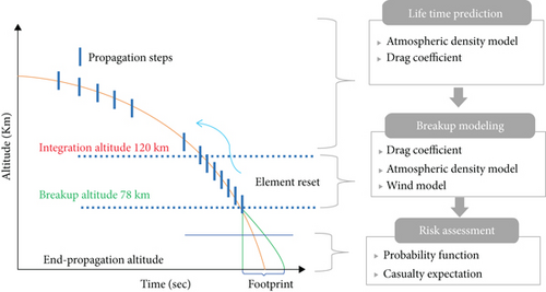
In the past 50 years, over 16,000 metric tons of man-made space objects and unexpected asteroids have entered the Earth’s atmosphere. Although most of them burn while entering the atmosphere, some of the debris have survived to impact the Earth’s surface and do expose a risk to people and property [1, 2]. To prevent these casualties, researchers have given considerable attention to the research area of reentry estimation of space objects. Usually, the starting altitude of a reentry object will be at around 120 km and then, breakup event happens at 78 km. However, the problem of estimation of space debris dispersion during the atmospheric reentry is still quite difficult due to unknown effects and uncertainties. Especially, the effects of atmospheric uncertainties are very difficult to determine since the atmospheric density and drag coefficient undergoes large fluctuations while decaying at that altitude [3]. In addition, the characteristics of uncontrolled space objects including the ballistic coefficients are largely insufficient to model the reentry trajectory. This is because the exact physical parameters of the objects like mass, area of cross section, shape, and dimensions are not available. Thus, the prediction of a reentry trajectory is generally estimated based on the statistical and stochastic method [4]. As shown in Figure 1, an estimated position and velocity vector of a reentering object is propagated by using a numerical integration model up to the breakup point at an altitude of 78 km. After the breakup occurred, the debris dispersion could be modeled by using various stochastic estimation approaches [5]. Several approaches for the estimation of the reentry time and impact locations have been proposed over the last decades [4–8]. For instance, Tardy and Kluever have estimated the states of orbital debris by using an optimal estimation method, and then Monte-Carlo simulation was carried out to predict the impact location with a final covariance matrix [5]. Reyhanoglu and Alvarado have proposed a Lyapunov equation-based covariance propagation method to predict the time evolution of debris trajectories [7]. In that method, a concept of positional probability ellipsoids is employed for the visualization of the time evolution of the debris dispersion. However, the Lyapunov equation-based covariance propagation method is based on the linearization of the translational equations of motion of the reentering space debris and the equations of the atmospheric reentry is subject to unknown uncertainties; thus, a high degree of neglected and truncated nonlinearities could lead to a degraded estimation of the debris dispersion [8, 9].
In order to compensate for the drawbacks of the Lyapunov-based estimation of the debris dispersion, alternative solutions could be employed by increasing the order of the Taylor-series expansion of the nonlinear system or by using an advanced numerical technique [9, 10]. These efficient alternatives include the unscented transformation [11], the divided-difference numerical integration [12–14], and the cubature quadrature integration [15]. As discussed in [11], the unscented transformation is able to capture the higher-order moments caused by the nonlinear transform better than the Taylor-series-based approximations used in the Lyapunov-based covariance propagation in [5]. The unscented transformation-based estimation technique is called the sigma point estimator [16, 17] in the sense that the estimator works on the principle that a set of deterministically sampled sigma points is used to parameterize the mean and covariance of the Gaussian random variables without the linearization step. The classification of the sigma point method is also interpreted as a special case of a weighted statistical linear regression (SLR) [18]. Even though the statistical linear regression approach and the unscented transformation approach could represent the estimation of the debris reentry trajectories, the estimation accuracy of the debris dispersion could be limited, because they capture the debris dispersion with the second-moment covariance using a fixed small number of sigma points extracted from a predefined covariance ellipsoid. Therefore, it is necessary to design an advanced approach which could include more precise distribution information of the debris dispersion and take into account the nonlinearities due to uncertain nonlinear motion of the reentering debris.
The main contributions of this paper are twofold. First, a precise and effective Gaussian cubature transformation-based [19, 20] estimation approach is proposed to compute the time evolution of the debris dispersion by using a moment-matching technique. The moment-matching formulation enables usage of many precise numerical integration methods such as Gauss-Hermite quadratures and cubature rules for multidimensional states [21]. In the Gauss-Hermite integration approach, a much larger set of sigma points and weights could be chosen compared to those of the Lyapunov covariance and the statistical regression approach such that with polynomial integrand the numerical approximation becomes exact and leads to more precise representation of the statistical moments (mean and covariance) of the distribution of a debris dispersion. Second, various parametric studies are carried out to analyze the effects of modeling uncertainties due to unpredictable atmospheric density and drag coefficients as well as wind effects near to the ground. For the analysis of the effects of the density model affecting the accuracy of the reentry prediction, four difference density models were used in the prediction of reentry trajectory. Specifically, NRLMSISE-00 [22], CIRA-72 [23], U.S. standard 1976, and exponential models [24] are compared with several different values of drag coefficient describing the unknown shape of breakup debris. During the atmospheric reentry, a time-varying empirical wind model is utilized to take into account a realistic environment, and it is based on HWM-07 (Horizon Wind Model 2007) [24, 25].
The remainder of this paper is organized as follows: Section 2 provides a description of the formulation of the reentry translational equations of motion. Section 3 provides two new approaches for the estimation and prediction of the debris dispersion due to the breakup during the reentry which is introduced by propagating the covariances of positional probabilistic ellipsoids. Section 4 shows performance comparisons of the proposed estimation approaches, that is, the statistical linear regression with the unscented transformation and the Gauss-Hermite cubature-based numerical approximation are demonstrated. Lastly, Section 5 provides a discussion of the simulation results.
2. Reentry Equations of Motion
2.1. Coordinate System
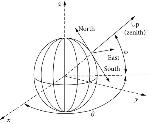
Let denote the topocentric horizon coordinate system at the breakup instant. The origin of this frame is at (θ0, ϕ0) on the Earth’s surface, where (θ0, ϕ0) denotes the initial longitude and latitude. The x1x2 plane is the local horizon, which is the plane tangent to the sphere at the origin. x3 is normal to this plane directed towards the zenith (i.e., the coordinate x3 is the geometric altitude). The x1 axis is directed eastward and the x2 axis points north. The x1x2x3 frame is also referred to as the ENU (east-north-up) coordinate [24] as shown in Figure 2.
2.2. Nonlinear Translational Equations of Motion
2.3. State-Space Nonlinear Equations of Motion
3. Algorithms for Estimation of Debris Dispersion
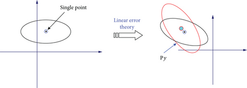
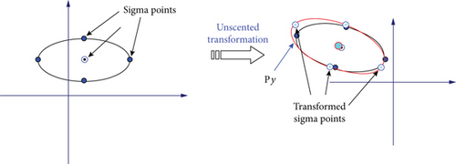
In this section, two new approaches for the estimation of debris dispersion due to a space vehicle breakup are proposed. The estimation of debris dispersion is represented in terms of a covariance propagation which describes probabilistic ellipsoids from a nominal reentry trajectory. First, a statistical linear regression using the unscented transformation is introduced to compute the time evolution of the covariance information. Second, a Gaussian moment-matching method which calculates the first and second moments of the probabilistic distribution of the debris dispersion by using a Gauss-Hermite cubature numerical approximation is proposed. Figure 3 depicts the difference between the conventional Lyapunov-based covariance approach and the unscented transformation-based covariance computation. In this work, detailed derivation for the covariance computation using the Lyapunov equation is not included but it can be referred to [5].
3.1. Statistical Linear Regression Approach for Estimation of Debris Dispersion
3.2. Gaussian Moment-Matching Approach for Estimation of Debris Dispersion
Even though the statistical linear regression (SLR) using the unscented transformation approach could represent the propagation of the debris dispersion due to a breakup event, the SLR-based approach estimates the debris dispersion with the second-moment covariance using a finite small number of sigma points. The statistical regression approach is not a truly global approximation and it does not work well with nearly singular covariances, that is, nearly deterministic systems with small covariances. For compensating the drawbacks, it is necessary to consider a more realistic approach which can precisely capture the initial debris dispersion and also take into account the neglected nonlinearities from the statistical linear regression. In this section, the Gaussian cubature transformation approach [10] is proposed to estimate the debris dispersion with a moment-matching technique by using a set of transformed sigma lattice points which represent breakup components in the debris dispersion (shown in Figure 4).
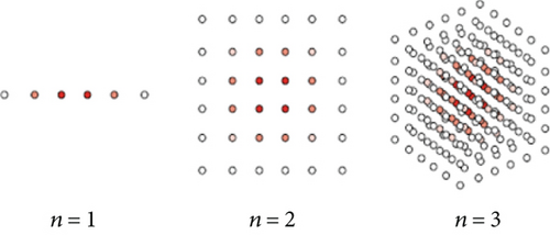
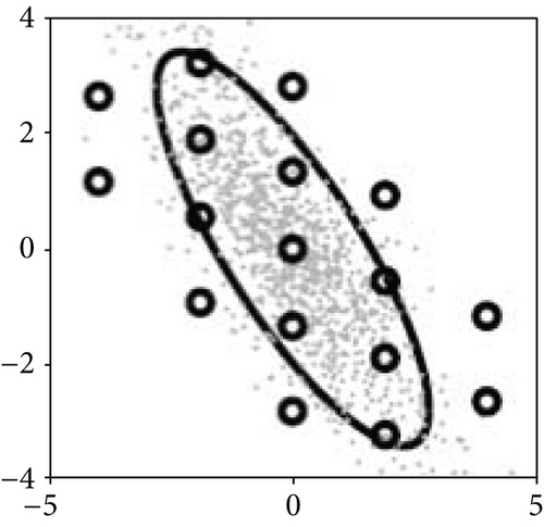
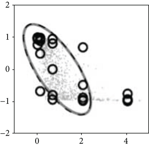
It is noted that the number of sigma points required for n-dimensional integral with pth-order rule is pn, which could become unfeasible when the number of dimensions grows which is indicated in Figure 4.
The multidimensional Gaussian-Hermite cubature-based covariance prediction approach which represents the debris dispersion and the distribution in time can be interpreted as a special form of a Monte-Carlo integration approach.
4. Simulation Results
In this section, first, various parametric studies are carried out to analyze the effects of uncertainties in the atmospheric density and drag coefficient along with wind effects. Then, the performance of the proposed estimation techniques are investigated by comparing two covariance propagation methods; the unscented transformation approach and the Gauss-Hermite cubature integration method.
4.1. Parametric Study for Analysis of Effects of Modeling Uncertainties
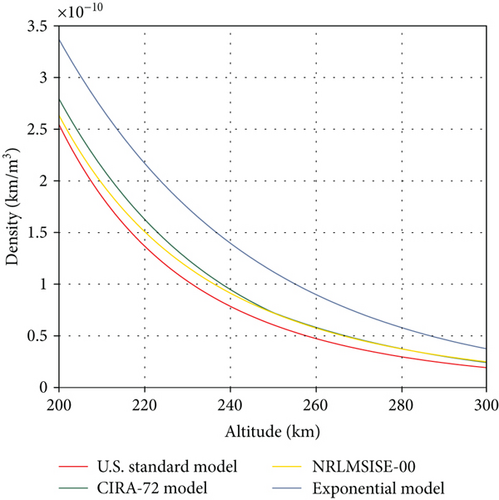
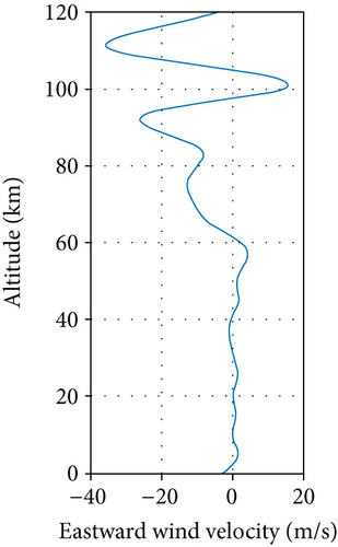
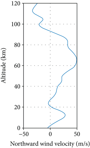
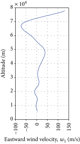
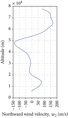
Atmospheric drag most strongly influences the motion of reentry objects near the Earth. When it comes to determining accurately atmospheric drag, the values of atmospheric density and drag coefficient are the main factors to the trajectory in the sense that the information on the specific shape and quantity of objects are generally unknown. In light of this reason, the different values of the drag coefficient are selected to see the how the drag coefficient affects the reentry point and the probabilistic ellipsoid of debris dispersion caused by the breakup event in this study. In this study, four different atmospheric density models including CIRA-72, Exponential model, U.S. standard model, and NRLMSISE-00 are used to analyze the effects of the atmospheric density model onto the reentry trajectory. Figure 6 shows density profiles corresponding to each density model as a function of altitude. Since wind also influences the reentry trajectory near to the ground, it is necessary to design a mathematical wind profile model. In this study, HWM-07 (Horizontal Wind Model 2007) [24] is employed to consider a more accurate reentry model. Figure 7 shows the velocity of eastward and westward winds with respect to the history of altitude.
In order to analyze the effects of the density model and the drag coefficient, two simulation examples are investigated. The first example considers the lifetime prediction of uncontrolled space objects with different atmospheric density models and drag coefficients. The satellite under consideration has the following orbit parameters: a = 6678 km, e = 1.0 × 10⁻⁵, i = 28.5°, ω = 0°, and Ω = 0°, and epoch time is defined as August 1, 2015. Figure 8 shows that the orbital decay of the space object until 78 km is different with respect to atmospheric models. Using the U.S. standard model, the decay of altitude is faster than any other density models. On the other hand, the NRLSMSISE-00 model predicts the decay of altitude of the reentry object with the slowest drop among the three models.
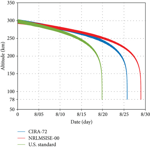
Table 1 presents the reentry latitude as well as longitude of different atmospheric models at the 78 km altitude and reentry time. Compared to the STK LTP (lifetime prediction) tool [26], it is shown that the results of reentry time are similar. Figure 9 indicates the orbital decay of space objects with a different drag coefficient. As the drag coefficient increases, it is shown that the space object falls faster.
| Density model | Reentry latitude | Reentry longitude | Reentry time | STK LTP tool |
|---|---|---|---|---|
| CIRA-72 | −38.936° | −345.39° | Aug. 26 (01:15) | Aug. 25 (18:21) |
| U.S. standard | −27.306° | −224.34° | Aug. 28 (15:44) | Aug. 27 (09:02) |
| NRLMSISE-00 | −8.302° | −319.91° | Aug. 20 (05:31) | Aug. 19 (03:22) |

The values of each latitude and longitude are taken with ϕi ∈ [−π/2, π/2) and θj ∈ [0, 2π), respectively, where i, j = 1, 2, …, 32 and Δv = 100 m/s is an incremental speed.
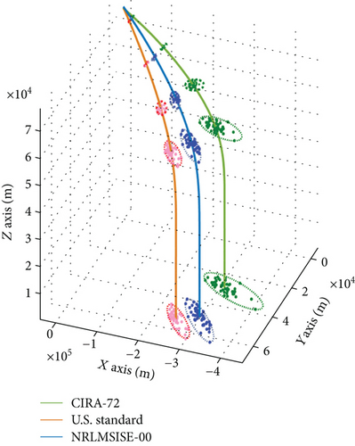
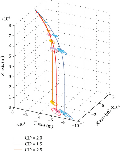
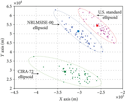
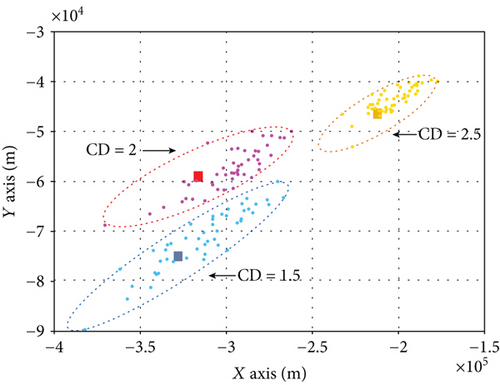
Figures 10 and 11 show the positional ellipsoid trajectory of breakup dispersion with different atmospheric density models and drag coefficients. As can be seen, even though each case of breakup event occurred at the same position, the final location of the ground impact point is very different depending on the type of the density model and the drag coefficient. Figures 12 and 13 show the final location and size of the positional ellipsoid on the ground in detail. For the case of different atmospheric models, the CIRA-72 model generated the largest impact area of dispersion debris, while the NRLSMSISE-00 model showed a smaller one, which indicates that the CIRA-72 model is subject to a lot of uncertainty errors compared to that of the NRLMSISE-00 models. Table 2 describes the footprint statistics including impact areas. For the case of a different drag coefficient, the size of the final positional ellipsoid of debris dispersion becomes smaller as the values of drag coefficients increase. It is indicated that a higher drag coefficient value leads to a faster fall to the ground with a short evolution. As can be shown in Table 3, the positional ellipsoidal area of CD = 1.5 is almost twice larger than that of CD = 2.5. It is seen that a properly estimated drag coefficient is one of the main factors in the propagation of the probabilistic positional ellipsoid.
| Density model | Impact latitude | Impact longitude | Impact area |
|---|---|---|---|
| CIRA-72 | −3.007° | −240.2° | 1522 km2 |
| U.S. standard | −27.306° | −224.34° | 619.2 km2 |
| NRLMSISE-00 | −8.302° | −319.91° | 913.8 km2 |
| Drag coefficient | Impact latitude | Impact longitude | Impact area |
|---|---|---|---|
| CD = 1.5 | 12.23° | −137.3° | 1093 km2 |
| CD = 2.0 | −7.452° | −347.3° | 916.5 km2 |
| CD = 2.5 | −11.96° | −118.3° | 547.3 km2 |
4.2. Statistical Computation of Debris Dispersion with Covariance Estimation
Note that the initial breakup dispersion generated with an incremental speed Δv uniformly added to the nominal velocity v(t0) in every direction could enter the inside of the initial covariance and thus the initial debris dispersion at the breakup event is simulated as shown in Figure 14.
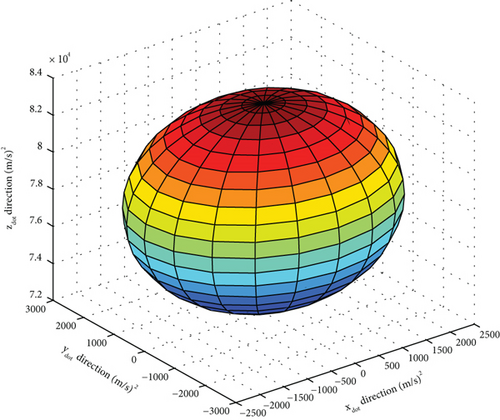
After the generation of the initial sigma points, the covariance is propagated by using (16), (17), and (18).
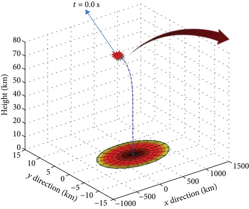
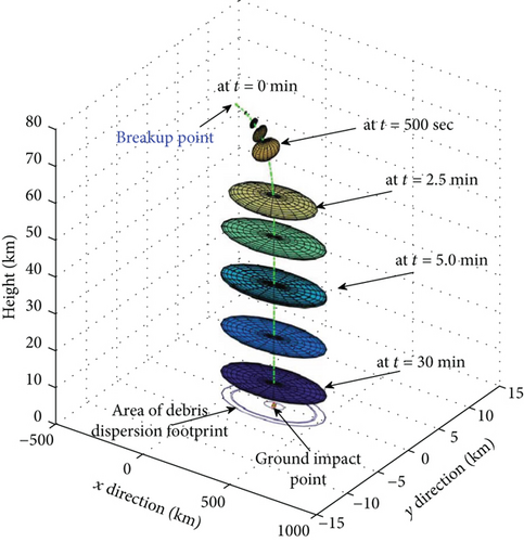
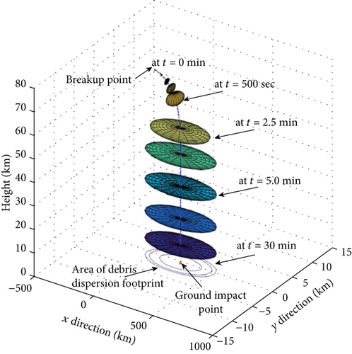
Figure 16 depicts the 3-dimensional positional probability ellipsoids corresponding to a confidence interval of 99.99% with a sequence of time instants. The breakup event during the reentry happened at the altitude of 78 km, and the predicted trajectory and the positional covariance ellipsoid of the debris fragments are well depicted with the usage of the proposed breakup dispersion estimation method. As can be shown, the positional probability ellipsoid representing the debris dispersion increases quickly within 2.4 minutes, and after 5 minutes the ellipsoid increases gradually until it impacts the ground. This phenomenon is understood by the fact that after 3 minutes from the breakup event the motion becomes a sharp fall and becomes nearly constant in motion.

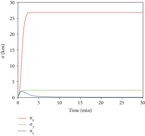
This phenomenon is verified in Figure 17 which shows the plots of the standard deviation of the positional covariance matrices in each direction over time. As can be expected from the time evolution of the debris dispersion in Figure 16, the variance sharply increases within 3 minutes but gradually changes after that time, that is, the falling motion 3 minutes after the breakup event.
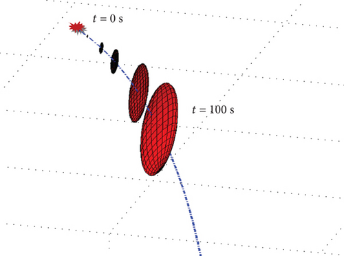
For a better analysis of the first few minutes, a detailed view is illustrated in Figure 18 which depicts the change of the initial debris dispersion in terms of the ellipsoid from the breakup event to 100 seconds. The covariance ellipsoid contains the debris fragments which are broken into all directions with the magnitude of the initial covariance matrix. For the first 100 seconds, the dispersion grows fast and becomes 10 times larger than the initial breakup ellipsoid. This indicates that right after the breakup event there are lots of uncertainties acting on the motion of the instantaneous debris dispersion and also the motion is highly nonlinear. A commonly used metric for covariance matrices is the square root of the trace of the covariance ellipsoid as seen in Figure 17.
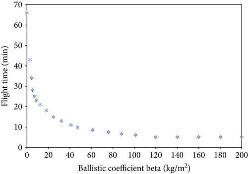
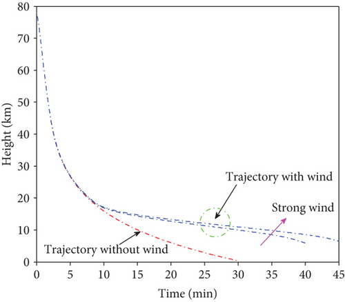
The simulation is made with different ballistic coefficients using the empirical density and wind models. Figure 19 shows the plot of flight time versus ballistic coefficient. In Figure 19, for the variance of the ballistic coefficient in terms of altitude, an empirical density profile obtained from the MSISE-00 density model [22] is used. In addition, in order to include the effects of wind near the ground, a wind model is developed by using a piecewise cubic spline method through a curve fitting of real wind data. Figure 20 represents the wind profiles used in the simulation in the eastern and northern direction as a function of different altitudes. The wind model used in this work is based on HWM-07 (Horizon Wind Model 2007) [7, 24]. Figure 21 illustrates the effects of the wind strength onto the time variation of the dispersion trajectory. As can be seen, if the strength of the wind is stronger, then it takes a longer time until the debris arrives the ground and impact it.
4.3. Performance Comparison for Estimation of Debris Dispersion
In this section, the performance of the proposed covariance methods for estimating the debris dispersion due to the reentry breakup is investigated in terms of the time evolution of the positional probabilistic ellipsoid. The covariance propagation methods include the unscented transformation-based statistical linear regression and the Gauss-Hermite cubature-based numerical integration methods described in Section 3.
For the simulation test, it is also assumed that the breakup altitude is 78 km and the initial breakup position is located at . The initial breakup dispersion is modeled as a Gaussian distribution with the initial covariance ellipsoid as given in (34); the process noise covariance matrix representing modeling uncertainties is also given by in (35). Now, based on the initial debris dispersion covariance matrix P(t0) and the process noise matrix Q(t), a set of sigma points representing a set of breakup components can be generated by using (14) for the unscented transformation (UT) method and using (29) for the Gauss-Hermite cubature (GHC) method. After the generation of the initial sigma points for the initial debris dispersion, the covariance is propagated by using (16), (17), and (18) for the UT method and (30), (31), and (32) for the GHC approach. The total simulation time used was 32 minutes.
Figure 22 depicts the estimated nominal trajectory from the breakup event to the ground impact instant, and also the footprint of the ground impact location. After the breakup event of the space debris during reentry, it is assumed that the simulation starts at t = 0 at the event, and then the nominal trajectory in terms of the mean value of all the debris fragments and the 3-dimensional positional ellipsoid are propagated until the debris fragments reach the ground. Based on the result in Figure 22, it is seen that the time evolution of the nominal estimates of the debris dispersion have different final locations but the overall trajectories are similar to each other. The nominal trajectory generated by the Gauss-Hermite cubature method has a little bit faster fall into the ground. The locational difference between the final footprint impact locations of two different methods was about 2 km in the x direction, and 10 m in the y direction, that is, . It is seen from the nominal trajectory plot that the uncertainties of the motion of the debris dispersion are captured more precisely by utilizing the Gauss-Hermite cubature technique compared to the unscented transformation method, and this is because the GHC method adopts a much larger set of sigma lattice points at the initial debris dispersion which leads to a more precise estimation of the debris dispersion. In the simulation, it is also seen that the reentry motion is a nonlinear motion right after the breakup event, but from the altitude near the ground the motion has relatively small nonlinearities due to a vertical falling motion.

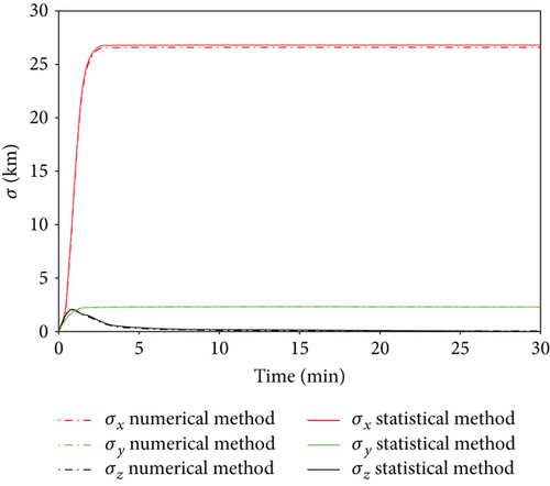
Figures 23 and 24 depict the profiles of the positional probability ellipsoids corresponding to a confidence interval of 99.99% for a sequence of time instants generated from the proposed covariance propagation methods, statistical linear regression, and the Gauss-Hermite moment-matching methods, respectively. In general, since the Gauss-Hermite cubature approach could include more debris breakup distribution points with p = 36 = 729 sigma points, it could generate a more accurate trajectory of the core debris as well as the covariance estimate of the breakup dispersion, while the unscented transformation method generates the initial breakup components with p = 2 × 6 + 1 = 13 sigma points. In addition, the performance of the proposed approach is investigated by checking the time evolution of the dispersion ellipsoid shown in Figures 23 and 24 where the time evolution of the positional probability ellipsoids can be seen to almost match between the statistical linear regression in Figure 23 and the Gauss-Hermite cubature-based numerical integration shown in Figure 24. In fact, the close agreement of these techniques can be justified by comparing the positional covariance matrices from both of the methods in each direction. It is seen that the size of the overall debris dispersion is similar to each other, 0.6 km in the x direction and 0.01 km in the y direction. Figure 25 shows the plots of the sigma values for the positional covariance matrices for both of the methods overtime. The difference of the sigma in the x direction is large but the other directions have similar values. The Gauss-Hermite cubature method could provide a little bit more accurate estimates of the nominal trajectory and the positional ellipsoid which could affect the calculation of the risk causality, but it also requires more computational power compared to the unscented transformation method. Both methods could satisfy the computational procedures required for real-time computation in a sequential estimation, while a Monte-Carlo-based approach uses offline computational procedures.
5. Summary and Conclusion
In this paper, for advanced analysis of the time evolution of space debris dispersion due to the breakup during reentry, two effective computational approaches were proposed to estimate the statistical distribution of the debris dispersion. The estimated debris dispersion is represented by using the prediction of positional probability ellipsoids for the visualization of the results. First, the time evolution of the covariance propagation was computed by using a statistical linear regression using the unscented transformation. Second, a novel covariance estimation technique was proposed by utilizing the Gaussian moment-matching method with a Gauss-Hermite cubature-based numerical integration approach. Compared to other covariance propagation methods, the newly proposed Gauss-Hermite cubature-based covariance computation could not only represent more exact initial dispersion, but also precisely calculate the time evolution of the debris dispersion with a large set of sigma points representing debris components. The Gauss-Hermite cubature approach does not require any linearization of the nonlinear translation equations of motion of a reentering debris, which leads to precisely taking into account nonlinearities exposed on the motion of a reentering debris. Furthermore, we also carried out a parametric study in order to analyze the effects on the accuracy of the covariance propagation due to modeling uncertainties. For the detailed parametric analysis, four types of density models and drag coefficients were used in the computation of the lifetime prediction and the covariance computation. In the simulation studies, it was shown that the newly proposed statistical linear regression method and the Gauss-Hermite computational approach are in close agreement to each other, but the Gauss-Hermite covariance propagation method provides a more precise estimate of the debris dispersion of the breakup fragments.
Conflicts of Interest
The authors declare that they have no conflicts of interest.
Acknowledgments
This study was supported by the Korea Astronomy and Space Science Institute (KASI) through the research project “Study on Precise Trajectory and Trajectory Uncertainty Prediction of Space Objects for Ground Impact Risk Assessment” (Project no. 2017-1-854-01) supervised by the Ministry of Science and ICT.


