For dynamic reliability design of complex structures with multiple components, an improved weighted regression distributed collaborative surrogate model method (IWRDCSMM) is developed from the extremum response surface method (ERSM), decomposed-coordinated thought, and improved weighted regression principle. The ERSM is used to address the dynamic reliability and sensitivity analyses of multicomponent structures and enhance the computing efficiency. The decomposed-coordinated thought is applied to handle the relationship among multiple components. The improved weighted regression method is used to find the efficient samples with smaller errors to improve the modeling accuracy. The proposed method is first introduced for dynamic probabilistic analysis (including reliability analysis and sensitivity analysis) of multicomponent structures. The method is then mathematically modeled by adopting the efficient samples selected based on the improved weighted regression method. Finally, the radial deformation dynamic probabilistic analysis of an aeroengine turbine blisk assembled by blade and disk is accomplished, in respect of the IWRDCSMM, fluid-thermal-structure interaction, and the randomness of input parameters within the time domain [0, T]. The results illustrate that the reliability degree of turbine blisk radial deformation is 0.9951 when the allowable value u_allow is 2.30 × 10⁻³ m, and all the input parameters affecting the turbine blisk radial deformation are gas temperature, angular speed, inlet velocity, outlet pressure, material density, and inlet pressure, successively. As revealed by the comparison of different methods, the IWRDCSMM has high fitting speed and simulation efficiency with the guarantee of accuracy. The efforts of this study provide a promising dynamic probabilistic analysis technique for complex structures with multiple components and enrich mechanical reliability theory.

1. Introduction

Mechanical system generally comprises multiple complex structures, and the complex structure is assembled by multiple components. For instance, turbine blisk in an aeroengine contains blade and disk [1]. Each structure plays a key role and is subjected to rigorous workloads during operation. The failure of complex structures easily results in the disorder of the whole mechanical system and even causes a catastrophic accident in the working process [2]. Therefore, it is required to investigate the probabilistic analysis of the complex structure to improve the performance and safety of the mechanical system with the consideration of the effects of dynamic loads. Probabilistic analysis generally includes reliability analysis and sensitivity analysis [3].

Lots of works have emerged on the probabilistic analysis. Chowdhury et al. [4] applied Monte Carlo (MC) simulation and finite element (FE) method to evaluate the reliability of the cracked structure. Naess et al. [5] employed MC simulation to estimate the reliability of the complicated structure considering the randomness of inputs. Tomasson and Soder [6] discussed the reliability evaluation of composite power systems using an improved way of applying MC simulation with the cross-entropy method. Jahani et al. [7] utilized interval MC simulation to perform the reliability analysis of the complex structure. Gao et al. [8] presented a mixed perturbation MC method for structural reliability analysis. Zhang et al. [9] studied multiobject reliability analysis of turbine blisk with multidiscipline under multiphysical field interaction by the MC method. Shayanfar et al. [10] sought a correction for the first-order reliability method by employing MC simulation to calculate the failure probability of a structure. Zhao and Ang [11] evaluated the reliability of the mechanical structure by the first-order third-moment method and random parameters. Alibrandi and Koh [12] used the first-order reliability method and secant hyperplane method to estimate the reliability of floating production systems. Lu et al. [13] used the second-order fourth-moment method to derive the structural reliability based on the first-order fourth-moment method [14]. Lin et al. [15] proposed the score function method with kernel density estimation for structural stochastic sensitivity analysis. All the above efforts complete the probabilistic analyses of the complex structure by only adopting direct simulation methods such as the MC method and first-order reliability method. Although it is precise for these methods, the computational burden is rather unbearable for most of the computing platforms.

To address the computational efficiency with the acceptable accuracy, the surrogate model method (also known as the response surface method (RSM)) was developed for probabilistic analysis. Cheng and Li [16] employed RSM to solve the inverse structural reliability problems with implicit functions. Allaix and Carbone [17] used an improved RSM to evaluate structural reliability. Fang and Tee [18] proposed a novel method for structural reliability analysis based on RSM and improved genetic algorithm. Li et al. [19] applied the RSM to fulfill the seismic reliability evaluation of steel-timber hybrid shear wall systems. Cheng and Liu [20] performed the reliability analysis of steel cable-stayed bridges based on the RSM. Zhang and Bai [21] presented extremum RSM (ERSM) to derive the dynamic reliability analysis of a two-link flexible robot manipulator. Lu et al. [22] developed multiple ERSM to finish the dynamic probabilistic analysis of an aeroengine turbine blisk assembled by disk and blade. Fei et al. [23–25] derived the ERSM-based least-squares support vector machine and demonstrated it to be efficient in the nonlinear dynamic probabilistic analysis of turbine components. Kaymaz and Gaspar et al. applied the Kriging model method to study the structural reliability analysis [26, 27]. Chojaczyk et al. [28] applied artificial neural network model to study the structural reliability analysis of steel structures. Lehky and Novak [29] used artificial neural network model to solve the inverse structural reliability problem. Cheng [30] integrated the advantages of the artificial neural network method, first-order reliability method, and importance sampling updating method for the serviceability reliability analysis of prestressed concrete bridges. The above efforts can accomplish the reliability and sensitivity analyses with acceptable efficiency, but the problem of unacceptable computational precision still exists since the limitation of quadratic polynomials is regarded as a surrogate model. Besides, these methods are only applicable to the probabilistic analysis of one component and one failure mode. Therefore, there is an urgent need for the dynamic probabilistic analysis of the multicomponent structure to develop an efficient method.

This paper is oriented to develop an efficient and accurate analytical method for the dynamic reliability design of the multicomponent structure by integrating the ERSM [23], decomposed-coordinated thought [31, 32], and the developed improved weighted regression method. This method is called improved weighted regression distributed collaborative surrogate model method (hereafter, IWRDCSMM). The ERSM is used to address the transient problem in the dynamic probabilistic analysis of the multicomponent structure to enhance the computing efficiency and accuracy. The decomposed-coordinated thought is applied to process the relationship among multiple components. The improved weighted regression method is used to find the samples with smaller errors or larger weight to improve the modeling accuracy. The model is adopted for the dynamic probabilistic analysis of the multicomponent structure within the time domain [0, T]. The dynamic probabilistic analysis of the radial deformation of the blisk is completed regarding fluid-thermal-structural interaction, to demonstrate the feasibility and reasonability of the proposed method.

The remaining of this paper is organized as follows. In Section 2, we elaborate the proposed IWRDCSMM. Section 3 applies this developed technique to the dynamic probabilistic analysis for the blisk radial running deformation, by considering the randomness of input variables of inlet velocity, inlet pressure, outlet pressure, gas temperature, material density, and angular speed. Section 4 verifies the feasibility and effectiveness of the method from the accuracy and efficiency of modeling and simulation by the comparison of the IWRDCSMM with other methods. Some conclusions on this study are given in Section 5.

2. Basic Theory

This section mainly introduces the basic theory of the IWRDCSMM. We first describe the procedure of the dynamic probabilistic analysis for multicomponent structure with the method. The details of ERSM and IWRDCSMM are then given in next two subsections. We finally discuss the thoughts of structural dynamic reliability and sensitivity analyses.

2.1. Procedure of Multicomponent Structural Dynamic Probabilistic Analysis

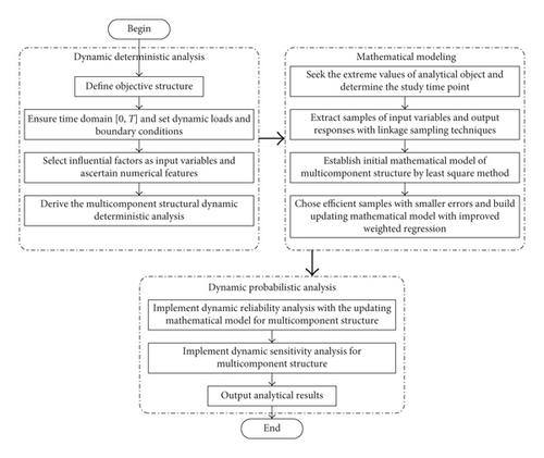
For the dynamic probabilistic analysis of multicomponent structure, IWRDCSMM is developed form ERSM, decomposed-coordinated thought, and improved weighted regression principle. The flow chart of multicomponent structural dynamic probabilistic analysis with IWRDCSMM is shown in Figure 1.

Details are in the caption following the image — **Figure 1**
Open in figure viewer PowerPoint

Flow chart of multicomponent structural dynamic probabilistic analysis with IWRDCSMM.

As illustrated in Figure 1, the procedure of multicomponent structural dynamic probabilistic analysis with IWRDCSMM mainly includes dynamic deterministic analysis, mathematical modeling, and dynamic probabilistic analysis. The details of this technique are summarized as follows:

(1)
Define objective structure with multicomponent, ensure analytical time domain [0, T], and set dynamic loads and boundary conditions.
(2)
Select influential factors as random input variables, ascertain their numerical features, and then derive the dynamic deterministic analysis of multicomponent structure.
(3)
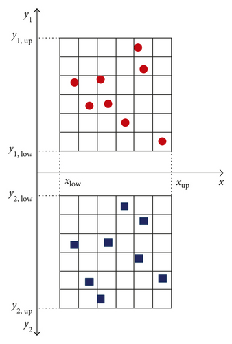
Find the extreme values of analytical object and determine the time point and obtain samples of input parameters and output responses with linkage sampling technique [9]. The linkage sampling method fuses the extremum selection method [33] and Latin hypercube sampling method [34, 35], which is defined as using a group input sample to obtain the output responses of multiple objectives at the same time. The linkage sampling method with one input parameter x and two output responses y₁ and y₂ is shown in Figure 2.
(4)
Establish the initial mathematical model of multicomponent structure by the least square method [22, 36, 37] based on the acquired samples and choose efficient samples with smaller errors or large weights which are selected from the acquired samples and the build updating model in line with improved weighted regression principle.
(5)
Implement the probabilistic analysis with the updating model for multicomponent structure.

2.2. Extremum Response Surface Method

ERSM is developed to simplify the process of output response of dynamic analysis within a time domain [0, T] as the extreme (maximum or minimum) value of process response, and then establish the extremum response surface model by fitting the acquired samples of random variable values and output extremum values. ERSM can thus reduce computing time and increase efficiency [21, 23, 36]. The mathematical model of this method is built in (1) with quadratic polynomial function, in which y_QP(x) indicates the extreme value of output response and x expresses the vector of input variables.

(1)

in which a is the unknown coefficient of constant, b is the vector of unknown coefficients of linear term, and c is the matrix of unknown coefficients of the quadratic term. Besides, b, c, and x can be written as follows:

(2)

where k is the number of input parameters.

Equation (1) is rewritten as quadratic polynomial function on basis of (2), that is,

(3)

in which a, b_i, and c_i are the unknown coefficients of the constant term, linear term, and quadratic term, respectively.

To obtain the unknown coefficients a, b_i, and c_i in (3), the least square method is used to fit the extremum response surface model. Its theory is denoted by

(4)

where w presents the vector of unknown coefficients, d expresses the matrix of input samples, and y indicates the vector of output response. w, d, and y are shown as follows:

(5)

where n is the number of samples of input parameters, and x_ik is the kth input parameter of the ith sampling date.

2.3. Improved Weighted Regression Distributed Collaborative Surrogate Model Method

ERSM can efficiently address the dynamic probabilistic analysis of single structure. However, it is difficult for this technique to resolve the dynamic reliability and sensitivity analyses of the multicomponent structure. Accordingly, the decomposed-coordinated thought is introduced into the ERSM, which is called as distributed collaborative surrogate model method (DCSMM) [37]. The multicomponent structure always refers to many subcomponents. We consider the structure with m subcomponents to investigate the DCSMM, and then the mathematical model of the DCSMM is established with respect to the least square method. The coordinated function can be written by

(6)

in which

is the decomposed function of the jth subcomponent and is expressed as

(7)

where a^(j) is the unknown coefficient of the constant term of the jth subcomponent,

the unknown coefficient of the linear term of the jth subcomponent,

is the unknown coefficient of the quadratic term of the jth component, and

is the value of the ith input sample of the jth subcomponent.

Despite the DCSMM reasonably handles the dynamic probabilistic analysis of the complex structure [37], the least square method is difficult to handle high-nonlinear function and large-scale samples in mathematical modeling. The conventional weighted regression principle is used to establish the mathematical model with few samples relative to the least square method. The weighted values are obtained by the ratio of the minimum output response to the output responses [38, 39]. The selected minimum output response may not be the optimal value, so that the fitting accuracy of mathematical model is unprecise. In this case, the improved weighted regression (IWR) method is developed to compute the weighted values by the ratio of the minimum error to the errors, and the efficient samples with smaller errors or larger weights are selected as the training samples of the fitting model. The errors are the absolute difference between the real value and the computing value. The minimum error is the minimum value of all obtained errors. The efficient samples are the samples with smaller errors or larger weighted values, selected from all samples. The IWR model is established using the selected efficient samples, the fitting performance of which is superiority to the least square method. The detailed validation procedure is stated in Section 4.

In the light of (6) and (7), the formula of the mathematical model of IWRDCSMM is

(8)

where

is the vector of efficient input samples,

is the value of the ith efficient input sample of the jth subcomponent,

represents the coordinated function that established the IWR,

indicates the decomposed function of the jth subcomponent with the IWR, and

, and

are, respectively, the unknown coefficients of the constant term, linear term, and quadratic term, which can be obtained via the IWR, that is,

(9)

in which

is the vector of unknown coefficients of the jth subcomponent for the IWRDCSMM,

is the matrix of input samples of the jth subcomponent,

is the weighted matrix of efficient samples, and

is the vector of output responses of the jth subcomponent.

, and

are shown in (10), and the weighted matrix

is defined by (11).

(10)

where

is the number of efficient samples.

(11)

in which

;

is the objective value of the jth subcomponent, namely, the minimum error,

is the

efficient output response of jth subcomponent by using the least square method, and

is the

efficient output response of jth subcomponent via the FE method.

Based on the above theories, the unknown coefficients in (8) are acquired, and the mathematical model of IWRDCSMM is established.

2.4. Dynamic Probabilistic Analysis

The IWRDCSMM is utilized to implement the dynamic probabilistic analysis (reliability analysis and sensitivity analysis) of complex structure with multiple components. In respect of the mathematical model of the IWRDCSMM, the limit state function of analytical object as

(12)

where Y_allow is the allowable value of analytical object,

is the vector of extracting input samples, and

is the value of the ith input variable of the jth subcomponent. Besides, the safety of complex structure is proved by

, and

indicates that the multicomponent structure failure.

To evaluate the dynamic reliability of multicomponent structure, the MC method is employed to achieve enough samples to obtain the values of limit state function with regard to (12) [40]. By the Chebyshev theorem and Bemoulli theorem [41] in probability theory, the structural failure and reliability probabilities are

(13)

in which N and N_f refer to the total number of extracting samples and the number of failures (as defined in (12) with a given Y_allow), respectively.

Sensitivity analysis of multicomponent structure can reflect the effect of the variation of input variables on failure probability or reliability probability, which help us determine the important degrees of input parameters on the output response of analytical object and then provide guidance for the design parameters of complex structures [1, 23, 40]. Sensitivity analysis typically contains sensitivity degree (S_d) analysis and impact probability (I_d) analysis [25]. Sensitivity degree reflects the influence level of an input variable on the output response, and impact probability indicates how much an input variable affects the output response relative to the other input parameters.

The sensitivity degree S_d is defined by the partial derivative of failure or reliability probability function with respect to the mean of input parameters, that is,

(14)

where χ is the reliability index, the distribution features of input variables obey normal distribution and are mutually independent. Therefore, ∂P_f/∂χ can be expressed by

(15)

in which

and

are the mean value and standard deviation of the limit state function, respectively.

Equation (14) is rewritten as follows:

(16)

The impact probability I_d is defined by the ratio of the absolute sensitivity degree of one input parameter to the sum of the absolute sensitivity degrees of all input variables, that is,

(17)

In addition, the relationship of the impact probability of all input variables is

(18)

In the light of the above analyses, the reliability degree and sensitivity indexes (sensitivity degree and impact probability) of random input variables on failure probability are acquired to evaluate the design quality of the complex structure.

3. Case Study: Dynamic Probabilistic Analysis of Turbine Blisk

In this section, the high-pressure turbine blisk of an aeroengine, which comprises blade and disk, is selected to demonstrate the proposed method in this paper. The dynamic probabilistic analysis of turbine blisk radial running deformation is accomplished to verify the feasibility and applicability in engineering practice, by considering the fluid-thermal-structural interaction.

3.1. Finite Element Model and Input Variables

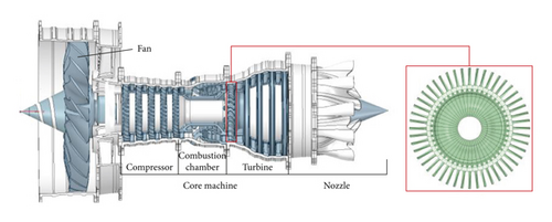
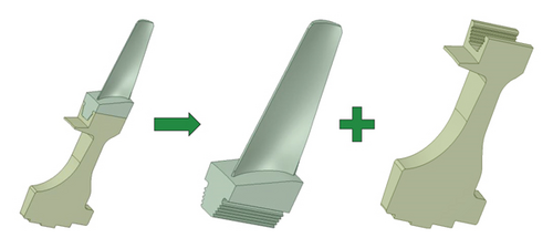
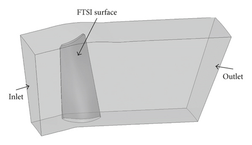
As an important structure of an aeroengine, high-pressure turbine blisk suffers high gas temperature and pressure from main combustion chamber and high centrifugal force due to angular speed. The schematic diagram of a blisk is shown in Figure 3. From Figure 3, it is obvious that the turbine blisk is a typical cyclic and symmetric structure. To save modeling burden and improve simulation time, 1/48 of the blisk model is selected as the object of study. The simplified three-dimensional models of the blisk and flow field are drawn in Figures 4 and 5, respectively. In Figure 5, the FTSI surface indicates the fluid-thermal-structural interaction surface which is to transfer fluid loads and thermal loads to the structure.

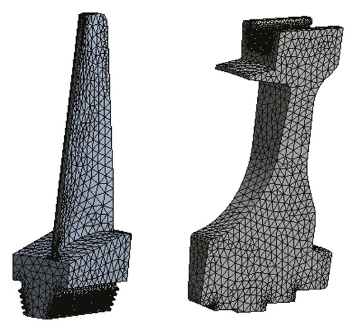
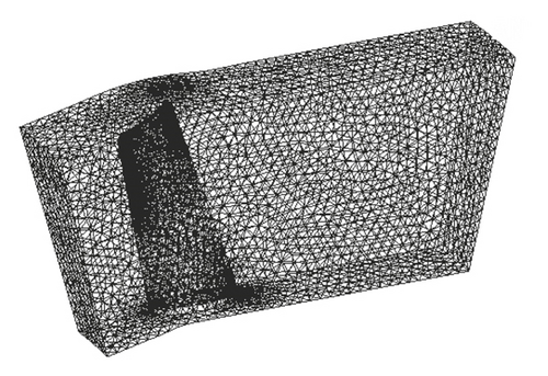
In view of Figures 4 and 5, the FE/FV models of turbine blisk and flow field are established in Figures 6 and 7, respectively. As illustrated in Figures 6 and 7, the FE models of turbine blade and disk are consisted of tetrahedrons with 48,551 elements, 75,097 nodes and 33,885 elements, 57,213 nodes, and the FV model of flow field has the tetrahedrons with 338,917 elements and 472,930 nodes.

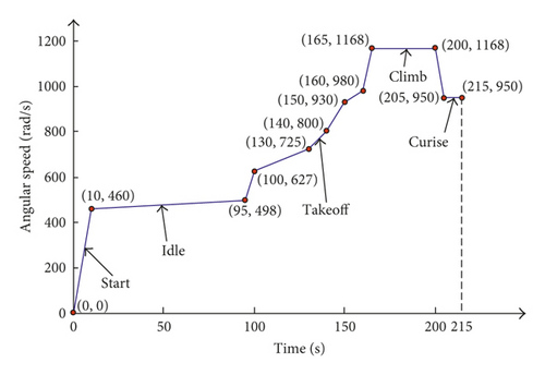
To study the influence of fluid-thermal-structural interaction on the radial deformation of turbine blisk, nickel-based superalloy GH4133 [42] is selected as the material of turbine blisk. The variation of angular speed within a time domain [0 s, 215 s] is shown in Figure 8. Here, 12 points are sampled as the calculation points [43]. The inlet velocity, inlet pressure, outlet pressure, and gas temperature are regarded as input variables to perform the deterministic analysis, and their means are assumed to be 160 m/s, 2 × 10⁶ Pa, 5.88 × 10⁵ Pa, and 1,200 K, respectively.

Substantially, the input variables process uncertainties and affect the blisk radial deformation, so that the randomness of input parameters needs to be considered. Therefore, the above parameters are regarded as random variables. Assuming that all random input variables obey normal distribution and are independent mutually; the distribution characteristics of the random variables are listed in Table 1.

Table 1. The numerical characteristics of these random input variables.

Variables	Distribution	Mean μ	Standard deviation σ
Inlet velocity, v (m/s)	Normal	160	3.2
Inlet pressure, p_in (Pa)	Normal	2 × 10⁶	4 × 10⁴
Outlet pressure, p_out (Pa)	Normal	5.88 × 10⁵	1.176 × 10⁴
Gas temperature, t (K)	Normal	1,200	24
Material density, ρ (kg/m³)	Normal	8,560	171.2
Angular speed, w (rad/s)	Normal	1,168	23.36

3.2. Dynamic Deterministic Analysis

Based on the determined values of input variables, the dynamic deterministic analysis of blisk radial deformation is carried out by the close-coupling analysis technique [22] with fluid-thermal-structural interaction. The procedure of dynamic deterministic analysis of blisk radial deformation contains fluid analysis, thermal analysis, structural analysis, and iterative solution.

The fluid analysis is based on the standard k-ε turbulence model with respect to the boundary conditions of the flow field and finite volume method. With regard to the thermal analysis, the law of energy conservation is utilized to resolve the property of turbine blisk flow flied, and then the pressure and gas temperature are transferred to turbine blisk through the FTSI surface. The structural analysis is performed by means of the FE method, in which the tetrahedron shape equation and geometric equation are applied to perform blisk radial deformation analysis. The dynamic deterministic analysis of radial deformation is finished by using the iterative solution.

According to the theory of the close-coupling analysis method, the dynamic deterministic analysis is accomplished, and the changing curves of the radial deformations of blade and disk with time are shown in Figure 9.

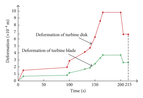
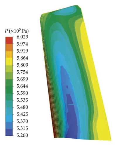
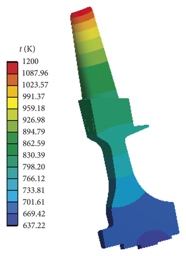
As shown in Figure 9, it is obvious that the radial deformation of turbine blisk increases with the increase of angular speed and the maximum emerges in the time domain [165 s, 200 s]. T = 175 s is chosen as the computing point. At this moment, the distributions of pressure on FTSI surface, temperature on turbine blisk, and the nephograms of blade and disk radial deformations are displayed in Figures 10–12, in which P indicates pressure, t expresses temperature, and u_b and u_d represent the radial deformations of blade and disk, respectively.

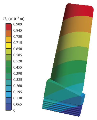
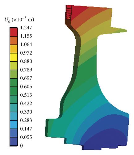
As illustrated in Figure 12, the maximum of radial deformation of turbine blisk occurs at the tip of blade and disk. Hence, the risk section responses of turbine blade and disk tip are selected as the output responses of the blisk and are also the maximum output responses of the blisk. The blisk is safe as the risk section is secure. Therefore, the output responses of turbine blade and disk tip are treated as the computational points in the blisk dynamic probabilistic analyses.

3.3. Derivation of Mathematical Model

To derive the IWRDCSMM model for the blisk radial deformation, the linkage sampling method is applied to extract 60 samples for random input variables following the numerical characteristics in Table 1. And then 60 samples for the corresponding output response are obtained by dynamic deterministic analyses. From this pool of 60 samples, 40 samples (as shown in Table 2) are selected to establish the initial mathematical model of blade and disk radial running deformations. The two models are displayed in (19). The remaining 20 samples are treated as the testing samples for the purpose of accuracy assessment.

Table 2. The training samples of input variables and output responses.

v (m/s)	p_in (×10⁶ Pa)	p_out (×10⁵ Pa)	t (K)	ρ (kg/m³)	w (rad/s)	u_b (×10⁻³ m)	u_d (×10⁻³ m)	Err_b (×10⁻⁶ m)	Err_d (×10⁻⁶ m)
153.94	2.075	5.762	1225.56	8698.60	1198.13	0.961	1.292	1.041	3.829	0.161	0.062
159.27	1.967	5.661	1163.76	8455.30	1122.44	0.904	1.207	1.158	4.312	0.144	0.055
147.73	1.902	5.844	1178.88	8598.03	1104.22	0.908	1.247	2.808	9.975	0.060	0.024
156.39	2.114	5.738	1238.16	8662.91	1130.85	0.967	1.273	1.673	6.615	0.010	0.036
148.39	1.912	5.973	1230.6	8526.67	1149.07	0.966	1.255	6.694	24.59	0.025	0.009
168.15	2.001	6.064	1188.9	8549.37	1168.70	0.921	1.275	4.823	17.96	0.035	0.013
155.50	2.111	6.002	1257.12	8604.52	1220.56	0.984	1.339	2.439	8.694	0.069	0.027
167.93	1.881	5.733	1230.12	8636.96	1217.75	0.968	1.296	2.534	9.045	0.066	0.026
150.39	1.938	5.834	1179.96	8611.01	1214.95	0.918	1.289	3.089	12.01	0.054	0.020
149.28	1.929	6.012	1191.24	8711.57	1158.88	0.931	1.248	1.865	6.947	0.089	0.034
152.39	1.895	5.781	1184.52	8633.72	1219.15	0.926	1.281	0.715	2.842	0.234	0.084
149.07	1.974	6.040	1253.94	8497.47	1118.24	0.975	1.285	0.934	3.518	0.178	0.068
153.28	1.941	6.021	1189.98	8478.01	1101.42	0.922	1.229	0.703	2.381	0.238	0.100
160.61	1.972	5.916	1222.62	8627.23	1123.84	0.951	1.267	0.388	0.239	0.431	1
151.51	2.118	5.676	1238.88	8406.64	1112.63	0.965	1.258	0.588	1.609	0.284	0.148
164.16	2.070	5.752	1222.14	8653.18	1143.47	0.950	1.279	1.673	6.128	0.099	0.039
163.49	1.922	5.930	1186.98	8461.79	1230.37	0.930	1.274	1.058	3.973	0.158	0.060
158.39	2.068	6.098	1173.72	8536.40	1164.49	0.909	1.260	4.719	18.38	0.035	0.013
148.62	1.994	5.704	1223.58	8649.94	1102.82	0.951	1.259	0.857	3.332	0.195	0.072
148.18	2.046	5.728	1208.1	8539.64	1139.26	0.944	1.244	5.296	19.75	0.032	0.012
153.06	1.984	5.810	1229.94	8578.57	1167.29	0.963	1.276	2.960	11.30	0.056	0.021
164.61	2.037	5.887	1147.74	8601.28	1185.52	0.894	1.235	2.274	8.451	0.073	0.028
168.82	2.058	5.647	1217.22	8630.47	1147.67	0.949	1.269	0.403	1.348	0.414	0.177
149.73	1.948	5.685	1222.02	8588.30	1165.89	0.949	1.297	5.475	19.84	0.031	0.012
161.27	1.910	5.920	1186.02	8429.35	1223.36	0.932	1.256	3.458	13.09	0.048	0.018
158.18	1.996	6.007	1183.62	8565.59	1121.04	0.915	1.248	2.699	9.584	0.062	0.025
163.05	2.030	5.988	1192.08	8409.88	1196.73	0.935	1.248	3.370	12.84	0.049	0.019
160.39	1.931	6112	1209.72	8646.69	1129.45	0.947	1.236	3.587	13.91	0.047	0.017
169.27	1.883	5.882	1234.86	8708.33	1132.25	0.960	1.287	3.253	12.08	0.051	0.020
152.62	2.003	5.872	1200.78	8413.13	1154.68	0.929	1.276	6.247	23.22	0.026	0.010
162.16	1.946	6.108	1169.34	8575.33	1216.35	0.913	1.266	1.908	6.999	0.088	0.034
163.72	1.898	5.829	1205.64	8435.83	1172.90	0.937	1.276	4.354	15.77	0.038	0.015
154.62	2.013	5.949	1201.44	8510.45	1235.97	0.939	1.301	1.051	3.649	0.159	0.065
164.83	2.063	6.026	1155.66	8500.71	1160.29	0.900	1.219	3.314	12.45	0.050	0.019
152.84	2.015	5.959	1157.22	8675.89	1175.70	0.899	1.251	1.935	7.252	0.086	0.033
150.62	1.917	5.968	1215.78	8458.54	1142.07	0.947	1.261	0.167	0.767	1	0.311
166.60	1.989	6.045	1183.74	8562.35	1182.71	0.927	1.242	4.745	17.35	0.035	0.014
166.16	2.025	6.055	1156.74	8594.79	1153.28	0.898	1.230	0.464	1.897	0.360	0.126
157.50	1.958	5.714	1194.54	8672.65	1199.53	0.937	1.265	1.675	5.936	0.099	0.040
169.49	2.056	5.642	1257.24	8507.20	1226.16	0.987	1.327	1.007	3.836	0.166	0.062

(19)

Based on (19) and (20), samples with smaller errors underlined and bold in Table 2 are chosen from 40 samples and are used to derive the IWRDCSMM model of blade and disk in (20).

(20)

3.4. Dynamic Probabilistic Analysis

In view of the IWRDCSMM model in (20), the limit state function of the blisk radial deformation is

(21)

where u_allow is the allowable value of radial deformation and

, and

are the extracting samples of input variables.

For the dynamic reliability analysis of blisk radial deformation, the allowable value u_allow is 2.30 × 10⁻³ m in respect of engineering experience. Based on the value and the limit state function, the MC method is applied to obtain 10,000 samples of input variables. The simulation history and histogram distribution of the blisk radial deformation are shown in Figures 13 and 14, respectively, in which u_max indicates the maximum of blisk radial deformation.

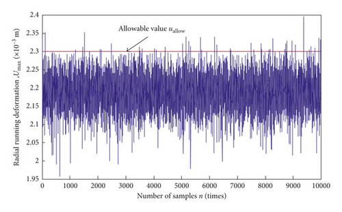
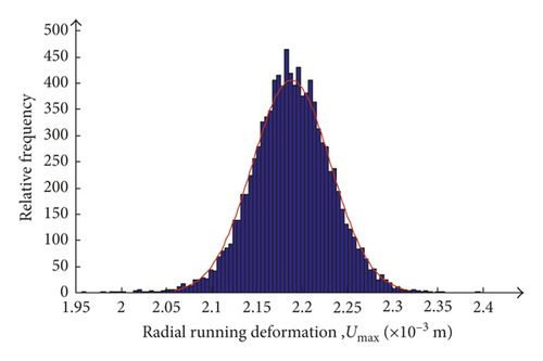
From Figures 13 and 14, it is obvious that the radial deformation of turbine blisk follows a normal distribution with the mean μ = 2.19 × 10⁻³ m and the variance σ² = 1.87 × 10⁻⁹ m. And the reliability degree R = 0.9951 is acquired, which satisfies the requirement of engineering design.

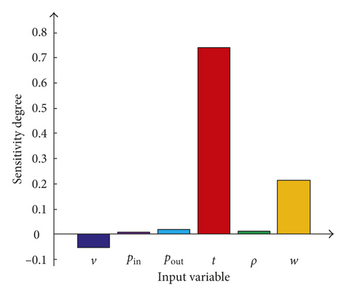
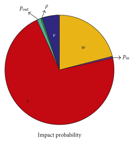
Additionally, the sensitivity analysis of blisk radial running deformation with respect to all input parameters is implemented. The analytical results including sensitivity degree and impact probability are obtained as depicted in Figure 15 and Table 3, respectively.

Table 3. Sensitivity degrees and impact probabilities of radial running deformation with all input variables.

Variable	Inlet velocity, v	Inlet pressure, p_in	Outlet pressure, p_out	Gas temperature, t	Material density, ρ	Angular speed, w
S_d	−0.054	0.004	0.012	0.740	0.006	0.216
I_d (%)	5.23	0.39	1.16	71.67	0.62	20.93

As demonstrated in Figure 15 and Table 3, the sensitivity degrees of all input parameters have either positive or negative values. The signs are related to whether the variation of an input variable has a positive or negative correlation with the output response [23, 33]. Hence, the blisk radial deformation increases with the increase of inlet pressure, outlet pressure, gas temperature, material density, and angular speed, while with the decrease of the inlet velocity. Besides, the impact probability reveals the importance of an input variable relative to other variables. The importance of all input parameters affecting the blisk radial running deformation are successively gas temperature, angular speed, inlet velocity, outlet pressure, material density, and inlet pressure.

In view of the above analysis, the effects of all input parameters on the blisk radial running deformation are acquired. This information might be used to guide the design of turbine blisk as well as update the model of the complex structure.

4. IWRDCSMM Verification

This section is to validate the effectiveness and feasibility of the developed IWRDCSMM. The fitting properties of both fitting efficiency and computing accuracy are firstly focused to validate the IWRDCSMM by comparing with distributed collaborative surrogate model method-based least square method (LSDCSMM) and distributed collaborative surrogate model method-based weighted regression principle (WRDCSMM). And then, these models and MC simulation are utilized to implement the dynamic reliability analysis of turbine blisk radial deformation to verify the superiority of the proposed method.

4.1. Fitting Property

This subsection is to verify the IWRDCSMM from the fitting property (including fitting efficiency and accuracy) perspective. The three models (LSDCSMM model, WRDCSMM model, and IWRDCSMM model) are built by the samples in Table 2. Therein, the forms of LSDCSMM and IWRDCSMM models are shown in (19) and (20). The formula of the WRDCSMM model is modeled in (22) with 20 samples by using conventional weighted regression principle [44, 45].

(22)

To support the IWRDCSMM model, the remaining 20 samples are selected as the testing samples. These models ((19), (20), and (22)) are verified by the below errors.

(23)

in which i = 1, 2, …, 20; u_i,test is the testing value of radial deformation for LSDCSMM, WRDCSMM, or IWRDCSMM corresponding to the ith sample; and u_i,true is the true value of radial deformation based on the FE model for the ith sample.

The analytical results including the fitting time and accuracy are listed in Table 4.

Table 4. Validation of fitting properties of IWRDCSMM with testing samples.

	Variables						LSDCSMM		WRDCSMM		IWRDCSMM
	v (m/s)	p_in (×10⁶ Pa)	p_out (×10⁵ Pa)	t (K)	ρ (kg/m³)	w (rad/s)	Values (×10⁻³ m)	Err. (×10⁻⁴ m)	Values (×10⁻³ m)	Err. (×10⁻⁵ m)	Values (×10⁻³ m)	Err. (×10⁻⁵ m)
Testing samples	157.05	1.951	5.757	1164.00	8448.81	1184.11	2.589	4.487	2.147	0.628	2.146	0.588
	154.83	1.970	6.031	1225.74	8523.42	1111.23	2.625	3.975	2.213	1.511	2.220	0.827
	160.83	1.914	5.700	1200.30	8581.81	1234.57	2.688	4.501	2.233	0.499	2.237	0.019
	149.95	2.073	5.906	1228.32	8643.45	1178.51	2.638	4.245	2.256	4.166	2.255	2.123
	162.82	2.102	6.103	1136.16	8481.25	1116.84	2.576	5.071	2.077	0.846	2.087	0.871
	161.05	2.104	6.069	1223.94	8494.23	1233.17	2.723	4.678	2.266	1.046	2.273	1.259
	165.71	1.943	5.743	1195.92	8555.86	1119.64	2.658	4.818	2.173	0.311	2.164	0.876
	159.94	1.886	5.863	1168.98	8503.96	1105.62	2.607	4.952	2.125	1.327	2.126	1.263
	151.06	2.099	5.901	1171.08	8400.15	1150.48	2.575	4.187	2.143	1.339	2.135	1.162
	147.51	2.032	5.925	1154.40	8666.16	1170.10	2.538	3.995	2.142	0.341	2.142	0.409
	149.51	1.893	5.652	1166.16	8529.91	1237.37	2.576	4.018	2.181	0.726	2.191	0.743
	162.38	1.934	5.944	1170.42	8484.49	1200.93	2.641	4.625	2.168	1.012	2.168	1.050
	165.93	2.006	5.772	1174.08	8465.03	1136.46	2.635	4.982	2.143	0.673	2.131	0.528
	161.49	2.094	5.776	1258.62	8422.86	1188.32	2.696	3.895	2.291	1.656	2.291	1.059
	153.72	2.051	5.815	1193.52	8559.11	1179.91	2.627	4.260	2.201	0.038	2.198	0.256
	155.94	1.900	5.805	1164.12	8487.74	1231.77	2.620	4.472	2.176	0.308	2.184	1.090
	163.93	1.986	5.935	1225.38	8546.13	1144.87	2.681	5.462	2.229	9.395	2.225	8.491
	161.94	2.020	6.084	1263.90	8490.98	1161.69	2.672	3.681	2.286	1.766	2.300	0.414
	155.72	2.044	5.853	1155.84	8682.38	1109.83	2.587	4.784	2.115	0.639	2.118	0.921
	169.04	2.027	5.997	1165.62	8640.21	1157.488	2.659	5.171	2.149	0.697	2.138	0.384
Absolute errors	Maximum, Err_max							5.462		9.395		8.491
	Minimum, Err_min							3.681		0.038		0.019
	Mean, Err_mean							4.513		1.446		1.167
Fitting time (s)								4.278		0.673		0.673

As revealed in Table 4, the fitting time of the IWRDCSMM model is less than that of the LSDCSMM model and is equal to that of the WRDCSMM model. The reason is that the number of samples for the IWRDCSMM is less than that of LSDCSMM and is equal to that of the WRDCSMM in mathematical modeling. The maximum absolute error, minimum absolute error, and average absolute error for the IWRDCSMM are only 0.155, 0.001, 0.026 and 0.904, 0.500, 0.807 for these of the LSDCSMM and WRDCSMM, respectively. The IWRDCSMM model holds less error and higher precision than the LSDCSMM and WRDCSMM.

4.2. Computational Property of Dynamic Reliability Analysis

To further validate the effectiveness and feasibility of the developed method, MC simulation, LSDCSMM, WRDCSMM, and IWRDCSMM are employed to perform the dynamic reliability analyses of turbine blisk radial running deformation based on the same input variables in Table 1 and computational environment. The computing time and precision of different simulations for different methods are listed in Tables 5 and 6.

Table 5. Computing time of turbine blisk dynamic reliability analyses with four methods.

Methods	Computing time (s)
Methods	10²	10³	10⁴
MC direct simulation	22,680,000	190,800,000	—
LSDCSMM	0.212	0.954	1.736
WRDCSMM
IWRDCSMM

Table 6. Analytical precision of turbine blisk dynamic reliability analysis with four methods.

Number of samples	Reliability degree R				Precision (%)
Number of samples	MC simulation	LSDCSMM	WRDCSMM	IWRDCSMM	LSDCSMM	WRDCSMM	IWRDCSMM
10²	0.99	0.96	0.97	0.99	93.94	97.98	1
10³	0.993	0.975	0.987	0.992	98.19	99.40	99.90
10⁴	—	0.9937	0.9945	0.9951	—	—	—

As shown in Table 5, in the computing time the IWRDCSMM is far less than the MC simulation and is equal to the LSDCSMM and WRDCSMM. In the computational efficiency, the IWRDCSMM becomes higher with the increasing simulations. As demonstrated in Table 6, the analytical precision of the IWRDCSMM is almost consistent with that of the MC simulation and is higher than those of LSDCSMM and WRDCSMM. As revealed in Tables 5 and 6, the proposed method can effectively accomplish the dynamic reliability analysis of complex structure with multiple components, while the MC simulation cannot when the number of simulation is over 10³.

In short, it is fully illustrated that the IWRDCSMM holds high precision and efficiency in modeling and simulation for the nonlinear transient reliability analysis of turbine blisk. The promising approach in this work is testified by the dynamic reliability and sensitivity analyses of complex structure with multiple components.

5. Conclusions

The main aim of this paper is to develop an improved weighted regression distributed collaborative surrogate model method (IWRDCSMM) with respect to the extremum response surface method (ERSM), decomposed-coordinated thought, and improved weighted regression (IWR), for the dynamic probabilistic analysis of complex structure with multiple components. The dynamic reliability and sensitivity analyses of the radial running deformation for an aeroengine turbine blisk comprising blade and disk are implemented by considering the influence of fluid-thermal-structural interaction to verify the effectiveness and feasibility of the proposed method. Some conclusions are acquired as follows:

(1)
Through the dynamic deterministic analysis of aeroengine turbine blisk, the changing rules of the blade and disk radial running deformations from start to cruise for aircraft are gained by adopting the close-coupling analysis technique within the time domain [0, T]. The turbine blisk radial running deformation reaches the maximum at t = 175 s.
(2)
The reliability degree of radial running deformation of turbine blisk is R = 0.9951 based on the dynamic reliability analysis of IWRDCSMM, when the allowable value of turbine blisk radial running deformation u_allow is 2.30 × 10⁻³ m.
(3)
From sensitivity analysis, the importance of all input parameters affecting the blisk radial deformation are successively gas temperature, angular speed, inlet velocity, outlet pressure, material density, and inlet pressure.
(4)
In fitting property, the IWRDCSMM needs smaller samples in modeling than other surrogate models and holds higher fitting efficiency and accuracy.
(5)
By the comparison of different methods, the proposed IWRDCSMM is promising to enhance computing efficiency with the guarantee of acceptable analytical precision in the dynamic probabilistic analysis of multicomponent structure.

Conflicts of Interest

The authors declare that there are no conflicts of interest regarding the publication of this article.

Acknowledgments

This study was supported by the National Natural Science Foundation of China (Grant no. 31601220), the School Cultivate Project Funding Scheme of Heilongjiang Bayi Agricultural University (Grant no. XZR2017-03), the Key Laboratory of Agricultural Mechanization Engineering, and The R & D Team for Sowing and Harvesting Equipment(Group no. TDJH201803). The authors would like to thank them.

Open Research

Data Availability

The data used to support the findings of this study are available from the corresponding author upon request.

References

1 Fei C. W., Choy Y. S., Hu D. Y., Bai G. C., and Tang W. Z., Transient probabilistic analysis for turbine blade-tip radial clearance with multi-component and multi-physics fields based on DCERSM, Aerospace Science and Technology. (2016) 50, 62–70, https://doi.org/10.1016/j.ast.2015.11.025, 2-s2.0-84955496985.
10.1016/j.ast.2015.11.025
Web of Science® Google Scholar
2 Song L. K., Wen J., Fei C. W., and Bai G. C., Distributed collaborative probabilistic design of multi-failure structure with fluid-structure interaction using fuzzy neural network of regression, Mechanical Systems and Signal Processing. (2018) 104, 72–84, https://doi.org/10.1016/j.ymssp.2017.09.039, 2-s2.0-85037811011.
10.1016/j.ymssp.2017.09.039
Web of Science® Google Scholar
3 Lu C., Feng Y. W., Liem R. P., and Fei C. W., Improved Kriging with extremum response surface method for structural dynamic probabilistic analysis, Aerospace Science and Technology. (2018) 76, 164–175, https://doi.org/10.1016/j.ast.2018.02.012, 2-s2.0-85042203092.
10.1016/j.ast.2018.02.012
Web of Science® Google Scholar
4 Chowdhury M. S., Song C. M., and Gao W., Probabilistic fracture mechanics by using Monte Carlo simulation and the scaled boundary finite element method, Engineering Fracture Mechanics. (2011) 78, no. 12, 2369–2389, https://doi.org/10.1016/j.engfracmech.2011.05.008, 2-s2.0-79960300010.
10.1016/j.engfracmech.2011.05.008
Web of Science® Google Scholar
5 Naess A., Leira B. J., and Batsevych O., Reliability analysis of large structural systems, Probabilistic Engineering Mechanics. (2012) 28, 164–168, https://doi.org/10.1016/j.probengmech.2011.08.024, 2-s2.0-84856548645.
10.1016/j.probengmech.2011.08.024
Web of Science® Google Scholar
6 Tomasson E. and Soder L., Improved importance sampling for reliability evaluation of composite power systems, IEEE Transactions on Power Systems. (2017) 32, no. 3, 2426–2434, https://doi.org/10.1109/tpwrs.2016.2614831, 2-s2.0-85018313090.
10.1109/TPWRS.2016.2614831
Web of Science® Google Scholar
7 Jahani E., Muhanna R. L., Shayanfar M. A., and Barkhordari M. A., Reliability assessment with fuzzy random variables using interval Monte Carlo simulation, Computer-Aided Civil and Infrastructure Engineering. (2014) 29, no. 3, 208–220, https://doi.org/10.1111/mice.12028, 2-s2.0-84892804593.
10.1111/mice.12028
Web of Science® Google Scholar
8 Gao W., Wu D., Song C. M., Tin-Loi F., and Li X. J., Hybrid probabilistic interval analysis of bar structures with uncertainty using a mixed perturbation Monte-Carlo method, Finite Elements in Analysis and Design. (2011) 47, no. 7, 643–652, https://doi.org/10.1016/j.finel.2011.01.007, 2-s2.0-79955472517.
10.1016/j.finel.2011.01.007
Web of Science® Google Scholar
9 Zhang C. Y., Lu C., Fei C. W., Liu L. J., Choy Y. S., and Su X. G., Multi-object reliability analysis of turbine blisk with multi-discipline under multi-physical field interaction, Advances in Materials Science and Engineering. (2015) 2015, 10, 649046, https://doi.org/10.1155/2015/649046, 2-s2.0-84943339001.
10.1155/2015/649046
Web of Science® Google Scholar
10 Shayanfar M. A., Barkhordari M. A., Barkhori M., and Barkhori M., Improving the first-order structural reliability estimation by Monte Carlo simulation, Proceedings of the Institution of Civil Engineers-Structures and Buildings. (2017) 170, no. 7, 532–540, https://doi.org/10.1680/jstbu.16.00208, 2-s2.0-85020251025.
10.1680/jstbu.16.00208
Web of Science® Google Scholar
11 Zhao Y. G. and Ang A. H. S., On the first-order third-moment reliability method, Structure and Infrastructure Engineering. (2012) 8, no. 5, 517–527, https://doi.org/10.1080/15732479.2010.539072, 2-s2.0-84862970412.
10.1080/15732479.2010.539072
Web of Science® Google Scholar
12 Alibrandi U. and Koh C. G., Stochastic dynamic analysis of floating production systems using the first order reliability method and the secant hyperplane method, Ocean Engineering. (2017) 137, 68–77, https://doi.org/10.1016/j.oceaneng.2017.02.031, 2-s2.0-85016423137.
10.1016/j.oceaneng.2017.02.031
Web of Science® Google Scholar
13 Lu Z. H., Hu D. Z., and Zhao Y. G., Second-order fourth-moment method for structural reliability, Journal of Engineering Mechanics. (2017) 143, no. 4, 06016010, https://doi.org/10.1061/(asce)em.1943-7889.0001199, 2-s2.0-85015883594.
10.1061/(ASCE)EM.1943-7889.0001199
Web of Science® Google Scholar
14 Liu Y., Lee T. X., Liu K., and Zhang Y. M., Chatter reliability prediction of turning process system with uncertainties, Mechanical Systems and Signal Processing. (2016) 66-67, 232–247, https://doi.org/10.1016/j.ymssp.2015.06.030, 2-s2.0-84955649890.
10.1016/j.ymssp.2015.06.030
Web of Science® Google Scholar
15 Lin S. P., Shi L., and Yang R. J., An alternative stochastic sensitivity analysis method for RBDO, Structural and Multidisciplinary Optimization. (2014) 49, no. 4, 569–576, https://doi.org/10.1007/s00158-013-1008-4, 2-s2.0-84897534178.
10.1007/s00158-013-1008-4
Web of Science® Google Scholar
16 Cheng J. and Li Q. S., Application of the response surface methods to solve inverse reliability problems with implicit response functions, Computational Mechanics. (2009) 43, no. 4, 451–459, https://doi.org/10.1007/s00466-008-0320-0, 2-s2.0-59449083248.
10.1007/s00466-008-0320-0
Web of Science® Google Scholar
17 Allaix D. L. and Carbone V. I., An improvement of the response surface method, Structural Safety. (2011) 33, no. 2, 165–172, https://doi.org/10.1016/j.strusafe.2011.02.001, 2-s2.0-79952773819.
10.1016/j.strusafe.2011.02.001
Web of Science® Google Scholar
18 Fang Y. F. and Tee K. F., Structural reliability analysis using response surface method with improved genetic algorithm, Structural Engineering and Mechanics. (2017) 62, no. 2, 139–142, https://doi.org/10.12989/sem.2017.62.2.139, 2-s2.0-85018632894.
10.12989/sem.2017.62.2.139
Web of Science® Google Scholar
19 Li Z., He M. J., Lam F., Zhou R. R., and Lee M. H., Seismic reliability evaluation of steel-timber hybrid shear wall systems, Earthquakes and Structures. (2017) 13, no. 3, 289–297.
Web of Science® Google Scholar
20 Cheng J. and Liu X. L., Reliability analysis of steel cable-stayed bridges including soil-pile interaction, Steel and Composite Structures. (2012) 13, no. 2, 109–122, https://doi.org/10.12989/scs.2012.13.2.109, 2-s2.0-84866436068.
10.12989/scs.2012.13.2.109
CAS Web of Science® Google Scholar
21 Zhang C. Y. and Bai G. C., Extremum response surface method of reliability analysis on two-link flexible robot manipulator, Journal of Central South University. (2012) 19, no. 1, 101–107, https://doi.org/10.1007/s11771-012-0978-5, 2-s2.0-84863065072.
10.1007/s11771-012-0978-5
Web of Science® Google Scholar
22 Lu C., Feng Y. W., Fei C. W., and Xue X. F., Probabilistic analysis method of turbine blisk with multi-failure modes by two-way fluid-thermal-solid coupling, Proceedings of the Institution of Mechanical Engineers Part C-Journal of Mechanical Engineering Science. (2017) In presshttps://doi.org/10.1177/0954406217723673, 2-s2.0-85045447477.
10.1177/0954406217723673
PubMed Web of Science® Google Scholar
23 Fei C. W. and Bai G. C., Nonlinear dynamic probabilistic analysis for turbine casing radial deformation based on extremum response surface method-based support vector machine, Journal of Computational and Nonlinear Dynamics. (2013) 8, no. 4, 041004, https://doi.org/10.1115/1.4023589, 2-s2.0-84878045440.
10.1115/1.4023589
Web of Science® Google Scholar
24 Fei C. W., Tang W. Z., and Bai G. C., Novel method and model for dynamic reliability optimal design of turbine blade deformation, Aerospace Science and Technology. (2014) 39, no. 6, 588–595, https://doi.org/10.1016/j.ast.2014.07.003, 2-s2.0-84911893863.
10.1016/j.ast.2014.07.003
Web of Science® Google Scholar
25 Fei C. W., Choy Y. S., Hu D. Y., Tang W. Z., and Bai G. C., Dynamic probabilistic design approach of high-pressure turbine blade-tip radial running clearance, Nonlinear Dynamics. (2016) 86, no. 1, 205–223, https://doi.org/10.1007/s11071-016-2883-1, 2-s2.0-84976313424.
10.1007/s11071-016-2883-1
Web of Science® Google Scholar
26 Kaymaz I., Application of Kriging method to structural reliability problems, Structural Safety. (2005) 27, no. 2, 133–151, https://doi.org/10.1016/j.strusafe.2004.09.001, 2-s2.0-10944263187.
10.1016/j.strusafe.2004.09.001
Web of Science® Google Scholar
27 Gasoar B., Teixeira A. P., and Soares C. G., Assessment of the efficiency of Kriging surrogate models for structural reliability analysis, Probabilistic Engineering Mechanics. (2014) 37, 24–34.
10.1016/j.probengmech.2014.03.011
Web of Science® Google Scholar
28 Chojaczyk A. A., Teixeira A. P., Neves L. C., Cardoso J. B., and Soares C. G., Review and application of artificial neural networks models in reliability analysis of steel structures, Structural Safety. (2015) 52, 78–89, https://doi.org/10.1016/j.strusafe.2014.09.002, 2-s2.0-84922271591.
10.1016/j.strusafe.2014.09.002
Web of Science® Google Scholar
29 Lehky D. and Novak D., Solving inverse structural reliability problem using artificial neural networks and small-sample simulation, Advances in Structural Engineering. (2012) 15, no. 11, 1911–1920, https://doi.org/10.1260/1369-4332.15.11.1911, 2-s2.0-84870716479.
10.1260/1369-4332.15.11.1911
Web of Science® Google Scholar
30 Cheng J., Serviceability reliability analysis of prestressed concrete bridges, Journal of Civil Engineering. (2013) 17, no. 2, 415–425, https://doi.org/10.1007/s12205-013-1374-x, 2-s2.0-84875512186.
10.1007/s12205-013-1374-x
Web of Science® Google Scholar
31 Fei C. W. and Bai G. C., Distributed collaborative probabilistic design for turbine blade-tip radial running clearance using support vector machine of regression, Mechanical Systems and Signal Processing. (2014) 49, no. 1-2, 196–208, https://doi.org/10.1016/j.ymssp.2014.04.013, 2-s2.0-84902548414.
10.1016/j.ymssp.2014.04.013
Web of Science® Google Scholar
32 Adomian G., A review of the decomposition method in applied mathematics, Journal of Mathematical Analysis and Applications. (1988) 135, no. 2, 501–544, https://doi.org/10.1016/0022-247x(88)90170-9, 2-s2.0-0041185368.
10.1016/0022-247X(88)90170-9
Web of Science® Google Scholar
33 Fei C. W., Bai G. C., and Chao T., Extremum response surface method for casing radial deformation probabilistic analysis, Journal of Aerospace Information Systems. (2013) 10, no. 1, 47–52, https://doi.org/10.2514/1.i010045, 2-s2.0-84875124683.
10.2514/1.I010045
Web of Science® Google Scholar
34 Olsson A., Sandberg G., and Dahlblom O., On Latin hypercube sampling for structural reliability analysis, Structural Safety. (2003) 25, no. 1, 47–68, https://doi.org/10.1016/s0167-4730(02)00039-5, 2-s2.0-0037212955.
10.1016/S0167-4730(02)00039-5
Web of Science® Google Scholar
35 Farzamian M., Monteiro S. F. A., and Khalil M. A., Constraining unsaturated hydraulic parameters using the Latin hypercube sampling method and coupled hydrogeophysical approach, Pure and Applied Geophysics. (2017) 174, no. 12, 4471–4487, https://doi.org/10.1007/s00024-017-1656-1, 2-s2.0-85036479987.
10.1007/s00024-017-1656-1
Web of Science® Google Scholar
36 Fei C. W., Bai G. C., Tang W. Z., and Choy Y. S., Optimum control for nonlinear dynamic reliability of the radial deformation of turbine casing with T-LSSVM, Advance in Materials Science and Engineering. (2015) 2015, 9, 680406, https://doi.org/10.1155/2015/680406, 2-s2.0-84924368645.
10.1155/2015/680406
Web of Science® Google Scholar
37 Bai G. C. and Fei C. W., Distributed collaborative response surface method for mechanical dynamic assembly reliability design, Chinese Journal of Mechanical Engineering. (2013) 26, no. 6, 1160–1168, https://doi.org/10.3901/cjme.2013.06.1160, 2-s2.0-84890848013.
10.3901/CJME.2013.06.1160
Web of Science® Google Scholar
38 Chi H. T., A discussion on the least-square method in the course of error theory and data processing, Proceedings of the 7th International Conference on Computational Intelligence and Communication Networks, December 2015, Jabalpur, India.
Google Scholar
39 Qiao B. Q., Liu S. M., Zeng H. D., Lee X., and Dai B. Z., Evaluation of dimension of fractal time series with the least square method, Science China-Physics Mechanics and Astronomy. (2017) 60, no. 4, 040521, https://doi.org/10.1007/s11433-016-9002-8, 2-s2.0-85013833967.
10.1007/s11433-016-9002-8
Web of Science® Google Scholar
40 Fei C. W. and Bai G. C., Distributed collaborative extremum response surface method for mechanical dynamic assembly reliability analysis, Journal of Central South University. (2013) 20, no. 9, 2414–2422, https://doi.org/10.1007/s11771-013-1751-0, 2-s2.0-84883876783.
10.1007/s11771-013-1751-0
Web of Science® Google Scholar
41 Nielsen A., The Monte Carlo computation error of transition probabilities, Statistics and Probability Letters. (2016) 118, 163–170, https://doi.org/10.1016/j.spl.2016.06.011, 2-s2.0-84989926768.
10.1016/j.spl.2016.06.011
Web of Science® Google Scholar
42 Gao H. F., Fei C. W., Bai G. C., and Ding L., Reliability-based low-cycle fatigue damage analysis for turbine blade with thermo-structural interaction, Aerospace Science and Technology. (2016) 49, 289–300, https://doi.org/10.1016/j.ast.2015.12.017, 2-s2.0-84954098872.
10.1016/j.ast.2015.12.017
Web of Science® Google Scholar
43 Lattime S. B. and Steinetz B. M., High-pressure-turbine clearance control systems: current practices and future directions, Journal of Propulsion and Power. (2004) 20, no. 2, 302–311, https://doi.org/10.2514/1.9255, 2-s2.0-1842787836.
10.2514/1.9255
Web of Science® Google Scholar
44 Kaymaz I. and McMahon C. A., A response surface method based on weighted regression for structural reliability analysis, Probabilistic Engineering Mechanics. (2005) 21, no. 1, 11–17, https://doi.org/10.1016/j.probengmech.2004.05.005, 2-s2.0-10844245456.
10.1016/j.probengmech.2004.05.005
Google Scholar
45 Xiong F. F., Liu Y., Xiong Y., and Yang S. X., A double weighted stochastic response surface method for reliability analysis, Journal of Mechanical Science and Technology. (2012) 26, no. 8, 2573–2580, https://doi.org/10.1007/s12206-012-0425-4, 2-s2.0-84866043230.
10.1007/s12206-012-0425-4
Web of Science® Google Scholar

Citing Literature

All articles

Dynamic Reliability Design of Multicomponent Structure with Improved Weighted Regression Distributed Collaborative Surrogate Model Method

Abstract

1. Introduction

2. Basic Theory