Optimal Rational Approximations by the Modified Fourier Basis
Abstract
We consider convergence acceleration of the modified Fourier expansions by rational trigonometric corrections which lead to modified-trigonometric-rational approximations. The rational corrections contain some unknown parameters and determination of their optimal values for improved pointwise convergence is the main goal of this paper. The goal was accomplished by deriving the exact constants of the asymptotic errors of the approximations with further elimination of the corresponding main terms by appropriate selection of those parameters. Numerical experiments outline the convergence improvement of the optimal rational approximations compared to the expansions by the modified Fourier basis.
1. Introduction
The first results concerning the convergence of the expansions by the modified Fourier basis appeared in the works [2, 8–10]. We present two theorems for further comparisons.
Under some additional requirements, the convergence rate is faster.
Theorem 2 (see [2], [10].)Assume f ∈ C2q+2(−1,1), f(2q+2) ∈ BV[−1,1], q ≥ 1, and f obeys the first q derivative conditions:
The main results of this paper are exact constants of the main terms of asymptotic errors and optimal parameters for improved pointwise convergence of rational approximations. First, we derive the exact estimates for the main terms of asymptotic errors without specifying parameters τc and τs. Second, we determine the optimal values of parameters τc and τs which vanish the main terms and lead to approximations with substantially better pointwise convergence rates. We found that optimal values of parameters and , k = 1, …, p, are the roots of some polynomials depending on p and q, where q indicates the number of zero derivatives in (8). Moreover, the choice of optimal parameters depends on the parity of p and also on the location of x, whether |x| < 1 or x = ±1.
For example, when p is odd and |x| < 1, the roots of the generalized Laguerre polynomial (see Appendix A) could be used for τc and τs. In this case, the convergence rate of the MTR-approximations is O(N−2q−p−[(p + 1)/2]−2) as N → ∞. It means better convergence compared to the expansions by the modified Fourier basis with improvement by factor O(Np+[(p + 1)/2]). When p is odd and x = ±1, the roots of the generalized Laguerre polynomial could be used. In this case, the convergence rate is O(N−2q−[(p + 1)/2]−1) with the improvement by factor O(N[(p + 1)/2]). The problem that we encountered is impossibility to get simultaneous optimality on |x| < 1 and at x = ±1. One must decide whether to use parameters that provide the minimal error on [−1,1], but with worse accuracy on |x| < 1, or work with optimal parameters on |x| < 1 with worse accuracy at x = ±1. We expose similar observations for even values of p.
The paper is organized as follows. Section 2 presents some preliminary lemmas. Section 3 explores the pointwise convergence of the MTR-approximations away from the endpoints when |x| < 1. Section 4 considers the pointwise convergence of the MTR-approximations when x = ±1. In these sections, we show also the results of numerical experiments which confirm and explain the theoretical findings. Section 5 presents some concluding remarks. Appendix A recalls some results concerning the Laguerre polynomials and Appendix B proves some combinatorial identities that we used in the proofs of lemmas and theorems.
2. Preliminaries
The following estimates can be simply obtained by means of integration by parts of the integrals in (3).
Lemma 3. Assume f ∈ C2m+1[−1,1], m ≥ 0, and f(2m+1) ∈ BV[−1,1]. Then, the following asymptotic expansions are valid:
Lemma 4. Assume f ∈ C2m+2[−1,1], m ≥ 0, and f(2m+2) ∈ BV[−1,1]. Then, the following asymptotic expansions are valid:
Lemma 5. Assume f ∈ C2q+p+r+1[−1,1], f(2q+p+r+1) ∈ BV[−1,1], q ≥ 0, r ≥ 0, p ≥ 1, and
Proof. In view of (12) and (26), we have
It remains to notice that for (see [20]). Hence, t − 2s ≥ w + p − k, and s ≤ [(t − w)/2].
3. Pointwise Convergence Away from the Endpoints
In this section, we explore the pointwise convergence of the MTR-approximations away from the endpoints. Next theorem reveals the asymptotic behavior of the MTR-approximations for |x| < 1 without specifying the selection of parameters τc and τs.
Theorem 6. Assume f ∈ C2q+p+2[−1,1], f(2q+p+2) ∈ BV[−1,1], q ≥ 0, p ≥ 1, and
Proof. We prove only estimate (44). Estimate (45) can be handled similarly.
Taking into account the fact that θk → 1 as N → ∞, we estimate only the sums on the right-hand side of (18). By the Abel transformation, we get
Note that Theorem 6 is valid also for p = 0 which corresponds to the modified Fourier expansions (compare with Theorems 1 and 2). In that case, the exact constants of the main terms in (44) and (45) coincide with similar estimate in [3] (Theorem 2.22, page 29).
Figures 1 and 2 show the behaviors of |RN| (p = 0) and |RN,p| (p = 1, 2, 3, 4), respectively, on interval [−0.7,0.7] for N = 64 while approximating (53). We used , k = 1, …, p in the rational approximations.
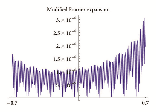
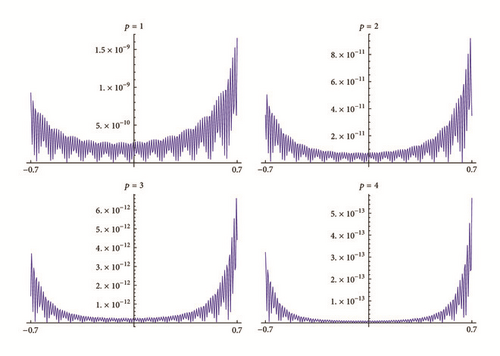
According to the results of Theorem 6, the bigger the value of p is, the higher the accuracy of the corresponding approximations is. We observe it empirically. We see that max[−0.7,0.7]|RN,p| is 3 · 10−8 for p = 0, is 1.6 · 10−9 for p = 1, is 9 · 10−11 for p = 2, is 6.6 · 10−12 for p = 3, and is 5.7 · 10−13 for p = 4.
Can we improve the accuracy of the rational approximations by appropriate selection of parameters τs and τc? Further, in this section, we give positive answer to this question and show how the optimal values can be chosen.
Next result is an immediate consequence of those observations and estimates of Theorem 6.
Theorem 7. Let f ∈ C2q+p+2[−1,1], f(2q+p+2) ∈ BV[−1,1], q ≥ 0, p ≥ 1, and
Theorem 7 is valid only if, for given p and q, polynomial (60) has only real-valued and nonzero roots. Further, we clarify this statement by showing those cases when it is true.
By imposing extra smoothness on the underlying functions, we derive more precise estimate of (62).
First, we need estimates for and .
Lemma 8. Assume f ∈ C2q+p+[(p + 1)/2]+2[−1,1], f(2q+p+[(p + 1)/2]+2) ∈ BV[−1,1], q ≥ 0, p ≥ 1, and
Proof. We prove only (64). By taking n = N in (33) and using (56), we get
Next theorem unveils the convergence rate of the MTR-approximations for odd values of p, when Qr(k) = Q0(k) ≡ 1. Note that, in this case, the roots of polynomial (60) coincide with the roots of generalized Laguerre polynomial (see Appendix A).
Theorem 9. Let parameter p ≥ 1 be odd, f ∈ C2q+p+(p + 1)/2+2[−1,1], q ≥ 0, f(2q+p+(p + 1)/2+2) ∈ BV[−1,1], and
Proof. We use (18) to estimate . The error can be estimated similarly.
Taking into account the fact that θk → 1 as N → ∞, we estimate only the sums on the right-hand side of (18). An application of the Abel transformation to the sums of leads to the following expansion of the error:
Taking into account the fact that (see (B.16))
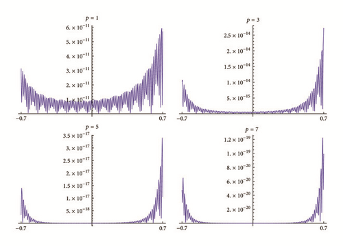
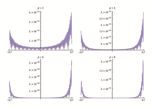
Figure 3 shows the result of approximation of (53) by the MTR-approximations with optimal parameters , k = 1, …, p as the roots of . We see better accuracy on [−0.7,0.7] compared to nonoptimal parameters as in Figure 2. For p = 1, the improvement is almost 25 times, and for p = 3, the improvement is almost 240 times.
Next theorem deals with even values of p. As we mentioned above, the best convergence rate is possible if Qr(k) = Q1(k) = 1 + c1k and τk, k = 1, …, p, are the roots of (60). We need to assume that polynomial (60) has only real-valued and nonzero roots x = zk, k = 1, …, p, for fixed p and q. In two cases, we can prove that it is true. When c1 = 0, the roots of polynomial (60) coincide with the roots of the generalized Laguerre polynomial (see Appendix A). When c1 = −1/(2q + 1 + p), the roots coincide with the ones of .
We saw from our experiments (which we cannot prove theoretically) that polynomial (60) has only real-valued and nonzero roots also for other values of parameter c1. However, based on our experiments, we observed that the rational approximations have almost similar accuracy for different values of c1 while approximating smooth functions on |x| < 1.
Theorem 10. Let parameter p ≥ 2 be even, f ∈ C2q+p+p/2+2[−1,1], q ≥ 0, f(2q+p+p/2+2) ∈ BV[−1,1], and
Proof. We prove only (80) and need only to estimate the sums on the right-hand side of (18). Similar to (71), we apply the Abel transformation and get the following expansion of the error:
According to (B.16), we have
Finally, from (84), we get
Theorems 9 and 10 conclude that by appropriate determination of parameters and , k = 1, …, p, we get extra improvement of the convergence rate of the MTR-approximations by factor O(N[(p + 1)/2]) compared to Theorem 6. Final improvement compared to the modified expansion is by factor O(Np+[(p + 1)/2]).
Let us return to MTR-approximations of (53). Figure 4 shows the results of approximation of (53) by the MTR-approximations with even p. Parameters , k = 1, …, p are selected as the roots of . Compared with Figure 2, we see better accuracy on |x| < 1. For p = 2, the improvement is almost 27 times, and for p = 4, the improvement is almost 200 times.
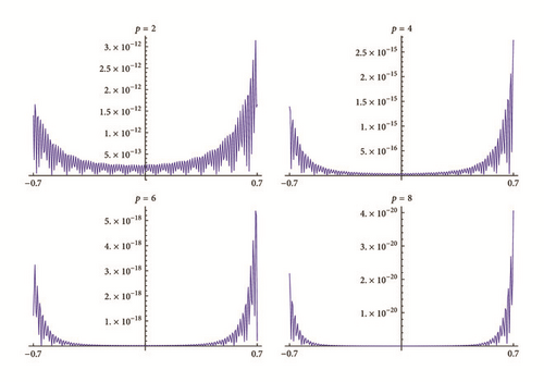
Figure 5 shows similar results with parameters , k = 1, …, p, as the roots of . In the next section, we will prove that those parameters provide improved accuracy also at x = ±1 for some p and q. We see that both choices of parameters provide similar results on |x| < 1.
4. Pointwise Convergence at the Endpoints
In this section, we explore the pointwise convergence of the MTR-approximations at the endpoints x = ±1. Next theorem explores the convergence of the rational approximations without determining parameters τc and τs.
Theorem 11. Assume f ∈ C2q+p+1[−1,1], f(2q+p+1) ∈ BV[−1,1], q ≥ 0, p ≥ 1, and
Proof. In view of (18) and (19), we write
Now, the proof immediately follows from the estimates of Lemma 5 by taking w = 0, r = 0 and by recalling that αp−k,p−k = (−1) p−k(p − k)!.
Note that this theorem is valid also for p = 0 which corresponds to the expansions by the modified Fourier basis (compare with Theorems 1 and 2).
Exact constants of the main terms in (90), for p = 0, can be found also in [10] (Theorem 3.2). We see that, in general, rational corrections do not increase the convergence rates of modified Fourier expansions at the endpoints x = ±1 without specifying appropriately parameters τc and τs. Both approaches have the same convergence rates O(N−2q−1).
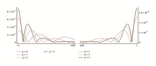
Moreover, as Figure 6 shows, without reasonable selection of the parameters, modified Fourier expansions have better accuracy compared to “nonoptimal” rational approximations at x = ±1.
Next theorem is the result of these observations and Theorem 11.
Theorem 12. Let f ∈ C2q+p+1[−1,1], q ≥ 0, p ≥ 1, f(2q+p+1) ∈ BV[−1,1], and
Note that Theorem 12 is valid only for those parameters p and q when polynomial (97) has only real-valued and nonzero roots. Further, we clarify this property with more details.
Our next goal is derivation of the exact convergence rate of (99).
Lemma 13. Assume f ∈ C2q+p+[(p + 1)/2]+1[−1,1], q ≥ 0, p ≥ 1, f(2q+p+[(p + 1)/2]+1) ∈ BV[−1,1], and
Proof. We prove only (102). In view of Lemma 5 (with w = 0) and (91), we write
By repeating the observations of previous section, it is possible to deduce that, for getting the maximal convergence rate for odd values of p, the polynomial Qr(k) can be at most degree 0 polynomial, Qr(k) = Q0(k) ≡ 1. For even values of p, Qr(k) = Q1(k) = 1 + d1k. In the first case, parameters τk are the roots of . In the second case, if d1 = 0, we get the roots of and if d1 = −1/(2q + p), we get the roots of . The next two theorems immediately follow from Lemma 13 and identity (B.12) and, we omit the proofs.
Theorem 14. Let parameter p ≥ 1 be odd, f ∈ C2q+p+(p + 1)/2+2[−1,1], q ≥ 0, f(2q+p+(p + 1)/2+2) ∈ BV[−1,1], and
Figure 7 shows the result of approximation of (53) by the rational approximations with optimal values of parameters τk, k = 1, …, p, as in Theorem 14. We see that, by increasing p (p is odd), we increase the accuracy of approximations at the points x = ±1. Note that p = 0 corresponds to the classical expansion by the modified basis and we see that, in contrary to Figure 6, the optimal choice of parameters do have big positive impact on the accuracy.
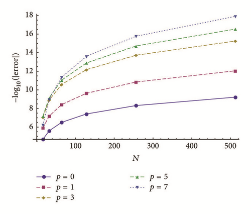
Comparison of Theorems 9 and 14 reveals the problem of the optimal rational approximations which is in the difference of optimal values of parameters τk for |x| < 1 and x = ±1. On |x| < 1 and x = ±1, the optimal values are the roots of and , respectively. The choice of will result in better accuracy on overall [−1,1] by the uniform norm, but on |x| < 1 the rate of convergence will be worse by factor O(N).
Next theorem explores even values of p.
Theorem 15. Let parameter p ≥ 2 be even, f ∈ C2q+p+p/2+2[−1,1], q ≥ 0, f(2q+p+p/2+2) ∈ BV[−1,1], and
Estimates (113) and (114) are valid if polynomial (112) has only real-valued and nonzero roots. As we mentioned above, in two particular cases when d1 = 0 and d1 = −1/(2q + p), the roots of the polynomial coincide with the roots of and , respectively. Both Laguerre polynomials have only real-valued and positive roots and Theorem 15 is valid in both cases. The choice of polynomial is reasonable as it will provide optimal rational approximation both on |x| < 1 (see Theorem 10) and at x = ±1 for some p and q.
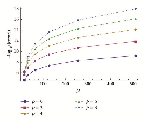
Figure 8 shows the result of application of the rational approximations to function (53) with optimal values of parameters τk, k = 1, …, p, as the roots of .
| q | 0 | 1 | 2 | 3 | 4 | 5 | 6 |
|---|---|---|---|---|---|---|---|
| −1 | 1 | 1/3 | 1/5 | 1/7 | 1/9 | 1/11 | |
| τ1 | −1.41 | 2.71 | 4.26 | 5.89 | 7.57 | 9.28 | 11.01 |
| τ2 | 1.41 | 13.29 | 11.74 | 13.31 | 15.29 | 17.39 | 19.53 |
| −3/14 | −3/2 | 3/10 | 3/22 | 3/34 | 3/46 | 3/58 | |
| τ1 | 0.12 | −27.44 | 2.61 | 3.81 | 5.10 | 6.45 | 7.85 |
| τ2 | 1.09 | 1.57 | 5.86 | 7.50 | 9.23 | 10.99 | 12.78 |
| τ3 | 3.46 | 4.44 | 10.85 | 12.72 | 14.76 | 16.86 | 18.98 |
| τ4 | 7.91 | 9.43 | 22.28 | 21.43 | 23.15 | 25.36 | 27.71 |
| −1/11 | −1/5 | 1 | 1/7 | 1/13 | 1/19 | 1/25 | |
| τ1 | 0.18 | −0.74 | 1.96 | 2.90 | 3.95 | 5.07 | 6.25 |
| τ2 | 1.00 | 1.34 | 4.28 | 5.57 | 6.98 | 8.46 | 9.98 |
| τ3 | 2.60 | 3.41 | 7.51 | 9.04 | 10.76 | 12.54 | 14.35 |
| τ4 | 5.15 | 6.45 | 11.99 | 13.62 | 15.55 | 17.59 | 19.67 |
| τ5 | 8.96 | 10.74 | 18.54 | 19.91 | 21.87 | 24.08 | 26.38 |
| τ6 | 14.84 | 17.18 | 75.72 | 31.25 | 31.35 | 33.32 | 35.69 |
| q | 0 | 1 | 2 | 3 | 4 | 5 | 6 |
|---|---|---|---|---|---|---|---|
| − | − | 1/2 | 1/4 | 1/6 | 1/8 | 1/10 | |
| τ1 | − | − | 4.417 | 6 | 7.653 | 9.347 | 11.07 |
| τ2 | − | − | 13.58 | 14 | 15.68 | 17.65 | 19.73 |
| −3/20 | −3/8 | 3/4 | 3/16 | 3/28 | 3/40 | 3/52 | |
| τ1 | 0.23 | −1.95 | 2.70 | 3.87 | 5.14 | 6.48 | 7.87 |
| τ2 | 1.35 | 1.83 | 6.09 | 7.63 | 9.31 | 11.05 | 12.83 |
| τ3 | 3.77 | 4.96 | 11.41 | 13.01 | 14.93 | 16.98 | 19.07 |
| τ4 | 8.249 | 10.16 | 35.80 | 22.99 | 23.76 | 25.69 | 27.92 |
| −1/14 | −1/8 | −1/2 | 1/4 | 1/10 | 1/16 | 1/22 | |
| τ1 | 0.20 | 0.53 | −16.59 | 2.94 | 3.98 | 5.09 | 6.27 |
| τ2 | 1.06 | 1.80 | 2.07 | 5.67 | 7.04 | 8.50 | 10.01 |
| τ3 | 2.71 | 3.88 | 4.52 | 9.23 | 10.86 | 12.60 | 14.40 |
| τ4 | 5.29 | 6.92 | 7.93 | 13.95 | 15.73 | 17.70 | 19.74 |
| τ5 | 9.14 | 11.23 | 12.62 | 20.58 | 22.21 | 24.28 | 26.52 |
| τ6 | 15.04 | 17.65 | 19.45 | 37.63 | 32.58 | 33.82 | 35.98 |
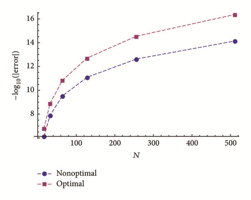
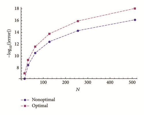
Figures 9 and 10 show the errors at x = ±1 while approximating (53) with rational approximations, where parameters and , k = 1, …, p, are selected according to Tables 1 and 2 for even and odd parts of the function, respectively. We called this approach “optimal” in the figures. For comparison, we showed also the result of approximations with parameters and , k = 1, …, p, as the roots of (see Figure 8 and Theorem 15). We called the latest “nonoptimal” in the figures. We see the impact of optimizations on the accuracy of the rational approximations at x = ±1.
The same approach can be applied also for the MTR-approximations and in that case all theorems of this paper will remain valid without the requirements of the derivatives at the endpoints x = ±1.
5. Conclusion
In this paper, we investigated the convergence of the MTR-approximations MN,p with parameters θc and θs defined by (24). The main goal of the paper was to show that by appropriate selection of parameters τc and τs it was possible to improve substantially the pointwise convergence of the approximations. We accomplished the main goal by calculating the exact constants of the main terms of asymptotic errors and by eliminating those constants through appropriate selection of the approximation parameters. We showed that the optimization depends whether |x| < 1 or x = ±1 and also whether parameter p is odd or even.
Theorem 6 provides general estimate on |x| < 1 proving that, without optimal selection of parameters and , k = 1, …, p, the rational approximations have convergence rate O(N−2q−p−2) as N → ∞ if an approximated function has enough smoothness and obeys the first q derivative conditions (see (8)). Compared with the modified Fourier expansions (see Theorems 1 and 2 or the same theorem with p = 0), the improvement is by factor O(Np) as N → ∞.
Theorem 9 gave the optimal choice for parameters τk when |x| < 1 and p was odd. If , k = 1, …, p, were the roots of the generalized Laguerre polynomial then the rational approximations had convergence rate O(N−2q−p−[(p + 1)/2]−2) with improvement by factor O(N[(p + 1)/2]) compared to nonoptimal choice of parameters (Theorem 6). The improvement was by factor O(N[(p + 1)/2]+p) compared to the expansions by the modified Fourier basis.
Theorem 11 imparts the convergence rate O(N−2q−1) of the rational approximations at x = ±1 without optimal selection of parameters. Comparison with Theorems 1 and 2 shows no improvement. Moreover, as our experiments show (see Figure 6) rational approximations without reasonable selection of parameters τk can perform worse at x = ±1 compared to the expansions by the modified Fourier basis.
Theorem 14 found the optimal values of parameters for odd p for better convergence rate at x = ±1. It proved that the best accuracy could be achieved when parameters were the roots of the generalized Laguerre polynomial . For that choice, the convergence rate was O(N−2q−[(p + 1)/2]−1) and improvement was by factor O(N[(p + 1)/2]) compared to the modified Fourier expansions.
We see that when p is odd, the optimal choices for |x| < 1 and x = ±1 are different. The choice of polynomial will provide the minimal uniform error on [−1,1], but, for |x| < 1, the convergence rate will be worse by factor O(N) compared to the optimal choice .
Conflicts of Interest
The authors declare that there are no conflicts of interest regarding the publication of this paper.
Acknowledgments
The research of the second author was supported by SCS Grant 16A-1a40.


