Downscaling of Open Coarse Precipitation Data through Spatial and Statistical Analysis, Integrating NDVI, NDWI, Elevation, and Distance from Sea
Abstract
This study aims to improve the statistical spatial downscaling of coarse precipitation (TRMM 3B43 product) and also to explore its limitations in the Mediterranean area. It was carried out in Morocco and was based on an open dataset including four predictors (NDVI, NDWI, DEM, and distance from sea) that explain TRMM 3B43 product. For this purpose, four groups of models were established based on different combinations of the four predictors, in order to compare from one side NDVI and NDWI based models and the other side stepwise with multiple regression. The models that have given rise to the best approximations and best fits were used to downscale TRMM 3B43 product. The resulting downscaled and calibrated precipitations were validated by independent RGS. Aside from that, the limitations of the proposed approach were assessed in five bioclimatic stages. Furthermore, the influence of the sea was analyzed in five classes of distance. The findings showed that the models built using NDVI and NDWI have a high correlation and therefore can be used to downscale precipitation. The integration of elevation and distance improved the correlation models. According to R2, RMSE, bias, and MAE, the study revealed that there is a great agreement between downscaled precipitations and RGS measurements. In addition, the analysis showed that the contribution of the variable (distance from sea) is evident around the coastal area and decreases progressively. Likewise, the study demonstrated that the approach performs well in humid and arid bioclimatic stages compared to others.
1. Introduction
Researchers agree on the key importance of precipitation data and its broad spectrum of use [1, 2]. In addition to its crucial role in the hydrological cycle balance, precipitation data is integrated into the assessment of extreme events, used as input in runoff and erosion modeling, utilized as an important parameter for hydrometeorological and agricultural hazards assessment, such as drought and flood. It is also one of the most challenging aspects of climate modeling. Precipitation is also a useful parameter in other fields such as ecology, natural resources, and environment.
Conventional measurements of precipitation in rain gauge stations (RGSs) allowed point-based estimations at specific geographic locations. The quality of the recorded precipitation data depends heavily on field observations, and the establishment of an adequate measuring network at the watershed level requires a nonnegligible cost (equipment, installation, maintenance, etc.). Furthermore, to consider the geographic variability of precipitation, one often relies on deterministic and geostatistical interpolation techniques such as IDW and Kriging. Although spatial interpolation techniques are widely used, they are hindered by several impediments [3] related to data precision, especially in watersheds where the number of RGSs is insufficient or inadequately distributed, as it is the case in developing countries [4].
The progress in open satellite precipitation products has relatively overcome this problem to some extent. Indeed, satellite missions such as TRMM (Tropical Rainfall Measuring Mission) and Climate Precipitation Center’s (CPC) morphing technique precipitation product (CMORPH) provide spatialized precipitation data with a coarse spatial resolution that is adequate for the characterization of large watersheds. Among the freely accessible data, one can mention TRMM 3B43, which is a monthly product, resulting from the combination of TRMM and other data sources (Huffman and Bolvin, 2014) [5, 6]. TRMM data is freely available at a spatial resolution of 0.25° for a period of 16 years, from 1999 to 2014 (https://disc.sci.gsfc.nasa.gov/alerts/nearing-the-end-of-the-trmm-era). Although TRMM data was restricted starting from October 7, 2014, due to the end of its fuel, this source of information still constitutes an important axis of research and is still applied in different studies [7–10].
TRMM 3B43 allows characterizing precipitation across large watersheds. However, the spatial resolution of this data is not fine enough to apprehend spatial variety over small and medium watersheds. For this purpose, different approaches are used to downscale this data to a fine resolution of 1 km [1, 11, 12]. Downscaling is of key importance in the field of remote sensing, since it allows an increase in spatial resolution [13]. Many downscaling techniques have been recently used in different fields and were reviewed by Jia et al. [12].
This study focuses on spatial downscaling of coarse satellite precipitation. This topic was recently studied by many researchers. Nichol and Abbas [10] studied the relationship between TRMM, at a spatial resolution of 0.25°, and Normalized Difference Vegetation Index (NDVI) at 1 km, in the Iberian Peninsula. The significant statistical relationship between these indicators allowed the downscaling of TRMM 3B43 products to a resolution of 1 km. A similar approach was used by Immerzeel et al. [11] to downscale the same product in the Qaidam Basin of China. During their analysis, TRMM 3B43 was downscaled using a multiple linear regression model, integrating NDVI and DEM [1, 11] downscaled version 7 of TRMM 3B43 over a humid and semiarid area, covering Lake Tana Basin in Ethiopia and Caspian Sea Region in Iran. The downscaling approach adopted in this study was based on a nonlinear relationship between the annual precipitation and the annual average of NDVI. The downscaled precipitation at 1 km was calibrated based on two approaches: Geographical Differential Analysis (GDA) and Geographical Ratio Analysis (GRA) [1]. In the same study, the researchers explored the disaggregation of monthly precipitation and demonstrated that the monthly downscaled precipitation has a good agreement with RGS measurements. Another strand of research has examined the downscaling of TRMM3B42 for six rainstorm events in the mountainous area of the Xiao River Basin in China [14]. The downscaling scheme was developed using multivariate regression that explains the precipitation by local topography and prestorm meteorological conditions. In this study, elevation, angle between slop aspect and prevailing wind, and the roughness index were used as a proxy of local topography, while antecedent maximum temperature and average humidity served as an indicator of prestorm meteorological condition [13]. The study showed a good agreement between downscaled precipitation and ground observation and revealed a better result than the conventional spline and Kriging interpolation methods.
The main objective of this study is to improve downscaled precipitation at a spatial resolution of 1 km using stepwise regression and Akaike’s Information Criterion (AIC), based on four predictors (NDVI, Normalized Difference Water Index (NDWI), elevation, and distance from sea). The specific objectives of this study are as follows.
Indeed, it has been shown that vegetation response has a positive relationship with precipitation at the annual scale (e.g., Malo and Nicholson, 1990; Martiny et al., 2006; Nicholson et al., 1990). This relationship was exploited to downscale annual TRMM precipitation using NDVI [1, 10]. With regard to NDWI, it could be a good proxy of precipitation and thus could be used to downscale TRMM 3B43, since it is sensitive to vegetation water content [15] (Gao, 1996). In this study, the potentialities of NDWI to desegregate TRMM 3B43 product will be explored, compared to those of NDVI, and evaluated using in situ measurements.
This study aims also to assess how stepwise regression and AIC could improve the models selection and thus downscaled precipitation. In this sense, desegregated precipitation through stepwise and AIC selected model was compared with those based on multiple regression using the four predictors (NDVI, NDWI, elevation, and distance from sea) and then evaluated through four statistical metrics estimated using independent in situ measurements (R2, RMSE, MAE, and bias).
Furthermore, the study investigated the contribution of distance from sea as a predictor to build robust regression models that could improve downscaled precipitation and assessed the sensitivity of the proposed spatial downscaled approach in five bioclimatic stages of the Mediterranean area.
2. Study Area
The study was carried out in Morocco, which is located in the southwest of the Mediterranean region, at the northwestern part of Africa. Morocco is bordered to the north by the Mediterranean Sea, to the west by the Atlantic Ocean, to the east by Algeria, and to the south and southeast by Mauritania (Figure 1). The country has a long coastline that extends for more than 3,500 kilometers.
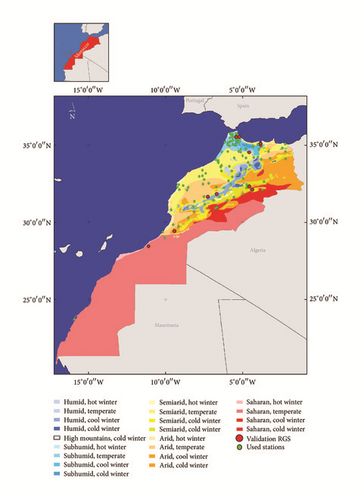
Morocco is essentially characterized by a Mediterranean climate, with mild and relatively wet winters and hot to dry summers. The climate shows enormous variations from subhumid in the north to Saharan in the south (Figure 1). This diversity is due to the combination of several factors, namely, its latitudinal location, the influence of the Atlantic Ocean and the Mediterranean Sea, and the influence of elevation through Atlas and Rif mountains. Spatial and temporal rainfall variability is considerably important. Mean annual rainfall ranges from less than 100 mm (Saharan bioclimatic stage) to 1200 mm (humid bioclimatic stage). The rainy season lasts from October to March in most of the country, and December, January, and February receive the maximum rainfall. The summer months have low rainfall and stormy character in general.
The total land area of Morocco is about 710850 km2, including 58000 km2 of forests (8%), 92000 km2 of agricultural lands (13%), and 460000 km2 of pastures, rangelands, and deserts.
3. Datasets and Methodology
3.1. Datasets
- (i)
A short time series of 15 years, from 1999 to 2012, of version 7 of TRMM 3B43 product. These images were collected in NetCDF format and used in this study.
- (ii)
NDVI and NDWI short time series of SPOT Vegetation (Satellite pour l’Observation de la Terre), from April 1998 to 2012, used in this research. This time series can be freely downloaded from SPOT Vegetation website (http://www.vito-eodata.be/PDF/portal/Application.html#Home). The Maximum Value Composites of the NDVI data over one or ten days, respectively, known as S10NDVI product, were used to generate monthly maximum value composite NDVI images and then to compute average annual NDVI images. The same approach was used in order to compute the average annual NDWI images on the basis of 10-day synthesis of NDWI.
- (iii)
Version 4.1 of Shuttle Radar Topography Mission (SRTM), which is available through the CGIAR-CSI Geoportal http://srtm.csi.cgiar.org/. The SRTM provides digital topographical data with a spatial resolution of 3 arc-seconds.
- (iv)
Map of distance, which was generated based on the coastline of the Atlantic Ocean and Mediterranean Sea using ArcGIS [16].
- (v)
A dataset of monthly rainfall data recorded in RGS, gathered from different sources and covering different periods between 1977 and 2012. Only the available data between 1998 and 2012 (period of acquisition of TRMM and SPOT Vegetation) were considered. During the first phase, the methodology was applied using a period of 6 years (1999–2004); after its validation, it was generalized to all the dataset (1999–2012). The number of the used stations varies from year to year in function of data availability. The number of the used stations during the first phase was 53, 61, 34, 34, 32, and 25 for the years 1999, 2000, 2001, 2002, 2003, and 2004, respectively.
- (vi)
A bioclimatic map: Emberger’s bioclimatic coefficient is a quite old classic concept [17, 18] (Emberger, 1955; Sauvage, 1963) that is still used in the Mediterranean area [19]. Emberger’s quotient (Q2) is used to define bioclimatic stages (per-humid, humid, subhumid, semiarid, arid, and Saharan) based on annual rainfall in mm (P), the average maxima of the hottest month (M), and the average minima of the coldest month (m) through this equation:
(1)
| Data | Period | Spatial resolution | Temporal resolution (synthesis) | Name of the variable |
|---|---|---|---|---|
| TRMM 3B43 | 1998–2012 | 0.25° | Monthly | TRMM |
| NDVI SPOT Vegetation | April 1998–2012 | 1 km | Decadal | NDVI |
| NDWI SPOT Vegetation | April 1998–2012 | 1 km | Decadal | NDWI |
| Altitude (SRTM V4.1) | 2008 | 90 m | — | Altitude |
| Distance from sea and ocean | 2014 | 1 km | — | Distance |
| Bioclimatic map | 1932 reviewed 1958 | 1/2,000,000 | — | — |
3.2. Methodology
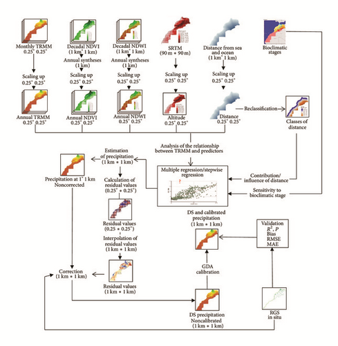
The adopted methodology in this study includes several steps (Figure 2). The main important ones are as follows.
3.2.1. Data Preparation
The monthly TRMM 3B43 precipitation was accumulated in order to calculate the annual TRMM precipitation year by year. Also, the zonal average of each predictor was calculated at a spatial resolution of 0.25°, to produce a dataset with the same spatial resolution. The same data preparation process was applied by Nichol and Abbas [10], by Zheng and Zhu [7], and by Duan and Bastiaanssen [1].
3.2.2. Comparison of the TRMM 3B43 and NDVI Relationship versus TRMM 3B43 and NDWI
For each year between 1999 and 2012, regression models were established using TRMM average annual precipitation as a dependent variable and NDVI as an independent variable. These models were compared to those performed using NDWI. Then, elevation and distance were integrated progressively in models, in a second and a third iteration.
3.2.3. Stepwise Regression and AIC Analysis
Stepwise multiple regression is a widely used approach to assess the importance of different predictors to explain a dependent variable. It is considered as a semiautomated process of building a model by successively adding or removing variables based on their estimated coefficients. The process of adding more variables stops when all of the variables have been included or when it is not possible to make a statistically significant improvement in R2 using any of the variables not yet included in the model. This statistical technique is applied in different fields including mathematics, Earth observation, and geoinformation [20–22].
It is worth mentioning that although it is a widely used approach by remote sensing and GIS community, stepwise multiple regression has several limitations, such as the bias arising from variable selection on the basis of statistical significance [23, 24]. To overcome these limitations, other model selection protocols are recommended. An interesting review of these techniques was given by Anderson et al. [25]. Among the techniques discussed by these authors, one can mention Akaike’s Information Criterion (AIC), Kullback–Leibler Information, and Takeuchi’s Information Criterion.
In this study, stepwise multiple regression and Akaike’s Information Criterion were applied in order to select the best combinations of variables (NDVI, NDWI, altitude, and distance from sea) that explain the maximum variation of TRMM and give the best models fit.
The stepwise multiple regressions were performed initially using a dataset of six years. These allowed choosing the most robust models for each year. Then, these models were double-checked and the best model fit for each year was selected using AIC. The resulting regression models using this approach led to a first group of models (Group 1) that were compared with a second group of models (Group 2), built on the basis of multiple regression using the same dataset. The models of two groups were evaluated using in situ measurement through four statistical metrics (R2, RMSE, MAE, and bias). This evaluation aims to assess whether the stepwise regression and the AIC improve the models fit and performance.
Using the same dataset, two other groups of models (Groups 3 and 4) were established. The models of Group 3 were built using stepwise regression integrating NDVI, altitude, and distance from sea, while the models of Group 4 were established using stepwise regression based on NDWI, altitude, and distance from sea. These two groups of models allowed us to compare and to evaluate downscaled precipitation using NDWI with those based on NDVI. The evaluation was undertaken through the same statistical metrics (R2, RMSE, MAE, and bias).
It is important to emphasize that the assumptions of normality, linearity, and homoscedasticity of the residuals were checked for all the selected models.
3.2.4. Downscaling and Calibration of TRMM Precipitation to 1 km
Three groups of models were used to downscale TRMM precipitation. This includes the selected models of Groups 2, 3, and 4. The selected models of Group 2 were chosen since they give a better fit compared to the models of Group 1. The selected models of Groups 3 and 4 were used to compare the contributions of NDWI and NDVI. The evaluation of three groups of models was based on the four statistical metrics mentioned above.
- (1)
The selected regression models were used to estimate the precipitation at a spatial resolution of 0.25° (PE0.25), in function of the predictors.
- (2)
Residual values of precipitation (RES0.25) were calculated at a spatial resolution of 0.25 by the difference between TRMM precipitation (TRMM0.25) and estimated precipitations (PE0.25). The residual values are considered as the amount of the annual precipitation that cannot be predicted by the models.
- (3)
The residual values (RES0.25) were interpolated to a spatial resolution of 1 km through the spline algorithm. This interpolation method estimates values using a mathematical function that minimizes the total surface curvature, resulting in a smooth surface that passes exactly through the sampled points [26]. Such algorithm is recommended when the punctual data is regularly spaced [10], as it is the case in this study. These interpolations allowed estimating the residual values at a fine resolution (RES1 km). The same interpolation approach was adopted by Immerzeel et al. (2009) and Duan and Bastiaanssen (2013).
- (4)
Preliminary estimations of downscaled precipitation were carried out by applying the regression models using the predictors at fine resolution (1 km), and then the results were corrected by adding the corresponding residual values (RES1 km).
- (5)
The Geographical Differential Analysis (GDA) [27] was adopted for the calibration of downscaled precipitation using RGS measurements. This approach was also used for the calibration of downscaled precipitation by Duan and Bastiaanssen [1]. The GDA relies on the in situ measurement at the level of rain gauge stations and was implemented year by year and model by model. In this sense, the difference between downscaled precipitation (DSP) and in situ measurement was calculated at the level of each gauge station. This difference is noted as the likely precipitation error (Perr). It was then interpolated via Inverse Distance Weighting algorithm, since the gauge stations are not regularly spaced. The final downscaled calibrated precipitation (DSC) was calculated by summing the downscaled precipitation (DSP) and the likely error (Perr) at a spatial resolution of 1 km∗1 km.
3.2.5. Comparison and Validation
It is worth noting that the same statistical metrics were used for the comparison of regression models of the three groups (2, 3, and 4). Likewise, the resulting downscaled precipitation was compared by visual interpretation. Also, after comparison and validation, the approach that gives the best model fit was used to extend the study to the other years (between 2005 and 2012).
3.2.6. Sensitivity to Mediterranean Bioclimatic Stages
The previously mentioned downscaled studies did not take into consideration the climatic zoning. In fact, the downscaled precipitation using the described scheme could be sensitive to climatic conditions, especially in the area where precipitation is low and/or denuded of vegetation. In this study, we explored this potential sensitivity in five bioclimatic stages of the Mediterranean area.
In this regard, it is worth mentioning that one of the key steps in the downscaling process is the establishment of robust regression equations, with the best fits. The regression models with low and statistically insignificant correlation coefficients will be unable to explain an important part of TRMM 3B43 product, and thus they cannot downscale it with accepted approximation. In this sense, the sensitivity of the proposed approach to the different bioclimatic stages can be assessed based on the statistical parameters of regression models. To this end, stepwise regression was performed year by year (1999–2004) for each of the five bioclimatic stages that characterize Morocco (humid, subhumid, semiarid, arid, and Saharan). The resulting regression models and their statistical parameters were compared over the five bioclimatic stages, year by year. The approach was considered sensitive to bioclimatic stage when the correlation coefficients are low and/or statistically not significant (p > 0.05). Downscaling of precipitation using these models could lead to unsatisfactory results. The approach was considered nonsensitive when the correlation coefficients are important and statistically significant.
3.2.7. Influence of Distance from Sea
The variable distance from sea was included in the original set of candidate models. However, the influence of distance could be important only in the first kilometers near the sea and not over all the study area. In addition, the area close to the Atlantic coast could be influenced by the sea breeze effect. To provide a better understanding of the influence and contribution of the distance from sea to explain TRMM product, a second analysis of this variable was performed. For this purpose, the map of this variable was classified into five classes, namely, Class 1 (0 to 0.25°), Class 2 (0.25° to 0.50°), Class 3 (0.50° to 0.75°), Class 4 (0.75° to 1°), and Class 5 (more than 1.00°). For each of these five classes, the stepwise regression was performed, year by year, using the four predictors. Then, the standardized coefficients of the distance from sea were compared class by class, year by years, using Tamhane’s post hoc test [29]. This allowed us to explore whether the contribution of the distance is significantly different across the five classes. The interval of 0.25° was chosen to be consistent with the spatial resolution of TRMM.
4. Results and Discussion
4.1. Relationship of TRMM 3B43 versus NDVI and NDWI
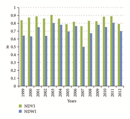
Figure 3 shows that TRMM versus NDVI and TRMM versus NDWI relationships have high R2 and all the selected models have a significant F-statistic. R2 ranges from to 0.70 to 0.82 for the TRMM versus NDVI and from 0.40 to 0.65 for the TRMM versus NDWI. Although the correlation between NDWI and TRMM is relatively moderate, they remain statistically significant. It can be concluded that both NDVI and NDWI can be used to explain TRMM 3B43.


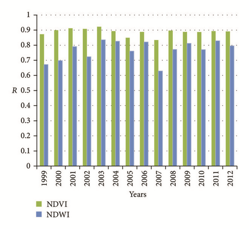
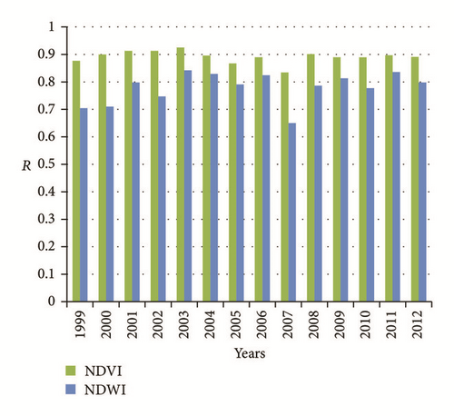
Figure 4 illustrates graphically that, after integrating the predictors elevation (Figure 4(b)) and distance (Figure 4(c)) in both NDVI and NDWI based models, all the correlation coefficients increase slightly and progressively. The lower limits of the correlation coefficients were increased from 0.76 to 0.83 for NDVI based models and from 0.51 to 0.63 for the NDWI, while the upper limits of the correlation coefficients increase slightly from 0.90 to 0.92 for the NDVI versus TRMM relationship and from 0.81 to 0.84 for the NDWI versus TRMM relationship.
The summary of unstandardized regression coefficients (B) of the NDVI, NDWI, elevation, and distance is given in Table 2. It can be seen that the unstandardized coefficients of NDVI and NDWI are higher than those of elevation and distance. This means that the NDVI and NDWI are the variables that contribute the most to the models. Elevation and distance have small unstandardized coefficients compared to NDVI and NDWI. By way of background, in addition to B, standardized regression coefficients are used in the interpretation of the contribution of the variable in the regression models. The standardized regression coefficients (Beta) refer to how many standard deviations a dependent variable will change, per standard deviation increase in the predictor variable. They are calculated by multiplying the unstandardized coefficient, B, by the ratio of the standard deviations for the independent and dependent variables. The use of Beta coefficients facilitates comparisons among independent variables since they are all expressed in standardized units. According to this analysis, it could be concluded that the statistical metrics of both NDVI and NDWI are significant; nevertheless, those of NDVI are better than NDWI. This can be explained by the fact that NDWI are more dynamic than NDVI; therefore, the NDWI syntheses do not capture all the variation of water content.
| Predictors | Unstandardized coefficients (B) | Standardized coefficients (Beta) | ||||||
|---|---|---|---|---|---|---|---|---|
| NDVI | NDWI | Distance | Elevation | NDVI | NDWI | Distance | Elevation | |
| Average | 1129.91 | 425.59 | −0.08 | 0.08 | 0.72 | 0.13 | −0.05 | 0.25 |
| SD | 188.52 | 217.72 | 0.04 | 0.02 | 0.05 | 0.06 | 0.03 | 0.05 |
- Average of significant models over the six years. SD: standard deviation.
According to Table 2, although the elevation has a small B, it is characterized by high standardized coefficients (Beta). This means that this variable has an important contribution to the regression models because they have a large absolute standardized coefficient (IBM Corp., 2012) The low values of Beta for the distance from sea indicate that this variable does not contribute significantly to the regression models. This may be explained by the fact that the influence of the sea could be important close to coastal areas and decreases with distance. The effect of distance was further analyzed in Section 4.5.2.
4.2. Stepwise Regression of TRMM and Predictors
It is important to recall that assumptions of normality, linearity, and homoscedasticity of the residuals were checked for all the selected models. Table 3 presents the statistical parameters of the models of Groups 1 and 2 that give the best model fit for the six years. As reported in Table 3(a), the six selected models by stepwise regression and AIC (Group 2) are characterized by high and statistically significant correlation coefficients (p < 0.001) and by very important unstandardized and standardized coefficients of the NDVI and NDWI. This means that NDVI and NDWI have an important contribution to the models (because they have a large absolute standardized coefficient). The variable elevation also contributes, to a lesser extent, to the models. Although its unstandardized coefficients are low, its standardized coefficients are relatively large, ranging from 0.21 to 0.32. Also, it should be noted that the unstandardized coefficients of these variables (NDVI, NDWI, and elevation) are positive, meaning that the precipitation increases as the values of these variables increase. Regarding the distance, it is characterized by negative standardized and unstandardized coefficients. This indicates that rainfall decreases as distance from the sea increases. However, the variable distance contributes slightly to the models, since the absolute values of their standardized and unstandardized coefficients are very small [30].
| Models | Years | R2 | Sig. | Unstandardized coefficients | Standardized coefficients | ||||||
|---|---|---|---|---|---|---|---|---|---|---|---|
| NDVI | NDWI | Distance | Elevation | NDVI | NDWI | Distance | Elevation | ||||
| Group 1: multiple regression models | 1999 | 0.78 | 0.000 | 802 | 307 | −0.11 | 0.07 | 0.67 | 0.13 | −0.09 | 0.30 |
| 2000 | 0.80 | 0.000 | 953 | 166 | −0.03 | 0.05 | 0.79 | 0.06 | −0.02 | 0.22 | |
| 2001 | 0.83 | 0.000 | 1344 | 635 | −0.05 | 0.08 | 0.70 | 0.18 | −0.03 | 0.22 | |
| 2002 | 0.84 | 0.000 | 1253 | 258 | −0.12 | 0.10 | 0.74 | 0.07 | −0.08 | 0.32 | |
| 2003 | 0.85 | 0.000 | 1216 | 401 | −0.11 | 0.07 | 0.75 | 0.13 | −0.05 | 0.20 | |
| 2004 | 0.82 | 0.000 | 1211 | 787 | −0.05 | 0.09 | 0.65 | 0.22 | −0.02 | 0.23 | |
| Group 2: stepwise regression models | 1999 | 0.78 | 0.000 | 802 | 307 | −0.11 | 0.07 | 0.67 | 0.13 | −0.09 | 0.30 |
| 2000 | 0.81 | 0.000 | 961 | 178 | — | 0.05 | 0.79 | 0.07 | — | 0.21 | |
| 2001 | 0.83 | 0.000 | 1355 | 654 | — | 0.08 | 0.71 | 0.18 | — | 0.21 | |
| 2002 | 0.84 | 0.000 | 1253 | 258 | −0.12 | 0.10 | 0.74 | 0.07 | −0.08 | 0.32 | |
| 2003 | 0.85 | 0.000 | 1216 | 401 | −0.11 | 0.07 | 0.75 | 0.13 | −0.05 | 0.20 | |
| 2004 | 0.83 | 0.000 | 1221 | 817 | — | 0.09 | 0.65 | 0.23 | — | 0.22 | |
| Models | Years | t | Tolerance | AIC | |||||||
|---|---|---|---|---|---|---|---|---|---|---|---|
| NDVI | NDWI | Distance | Elevation | Sig. | NDVI | NDWI | Distance | Elevation | |||
| Group 1: multiple regression models | 1999 | 30.77 | 5.80 | −4.65 | 15.03 | 0.000 | 0.530 | 0.514 | 0.609 | 0.628 | 9557 |
| 2000 | 38.30 | 3.04 | −1.12 | 11.99 | 0.263 | 0.514 | 0.532 | 0.611 | 0.670 | 9536 | |
| 2001 | 31.51 | 8.04 | −1.41 | 13.15 | 0.159 | 0.392 | 0.394 | 0.626 | 0.703 | 10247 | |
| 2002 | 37.30 | 3.64 | −4.34 | 19.30 | 0.000 | 0.469 | 0.456 | 0.582 | 0.672 | 9843 | |
| 2003 | 29.71 | 4.91 | −3.18 | 12.80 | 0.002 | 0.273 | 0.267 | 0.603 | 0.711 | 10146 | |
| 2004 | 26.88 | 8.85 | −1.21 | 4.89 | 0.228 | 0.344 | 0.317 | 0.572 | 0.669 | 10445 | |
| Group 2: stepwise regression models | 1999 | 30.77 | 5.80 | −4.65 | 15.03 | 0.000 | 0.530 | 0.514 | 0.609 | 0.628 | 9557 |
| 2000 | 39.90 | 3.32 | — | 13.63 | — | 0.550 | 0.554 | — | 0.964 | 9524 | |
| 2001 | 32.36 | 8.39 | — | 14.63 | — | 0.407 | 0.405 | — | 0.980 | 10205 | |
| 2002 | 37.30 | 3.64 | −4.34 | 19.30 | 0.000 | 0.469 | 0.456 | 0.582 | 0.672 | 9843 | |
| 2003 | 29.71 | 4.91 | −3.18 | 12.80 | 0.002 | 0.273 | 0.267 | 0.603 | 0.711 | 10146 | |
| 2004 | 27.13 | 9.58 | — | 15.27 | — | 0.347 | 0.345 | — | 0.976 | 10441 | |
- Sig.: signification test of distance from sea at 2-tailed p.
The models of Groups 1 and 2 were compared in order to assess whether stepwise regression and AIC improved the models through the selection of the appropriate variables and the best model fits. The comparison was based only on the years 2000, 2001, and 2003, since for the other years the models of Groups 1 and 2 are the same. It appears from Tables 3(a) and 3(b) that even though the correlation coefficients are more or less the same for the two groups of models, Student’s t absolute values are small and statistically not significant for the models of Group 1 that correspond to the years 2000, 2001, and 2004. The use of stepwise regression and AIC allowed addressing this constraint by selecting the “best” models that do not include the variable distance.
On the other hand, the AIC values are relatively low for the models of Group 2 compared to those of Group 1. This confirms that models of Group 2 perform relatively more than those of Group 1. Regarding the tolerance of the predictors, they range from 0.27 to 0.53 for NDVI, from 0.26 to 0.55 for the NDWI, from 0.58 to 0.62 for distance, and from 0.62 to 0.98 for elevation. This suggests that there is no significant multicollinearity in the regression models.
It can be concluded that the use of stepwise regression and AIC-based model selection allowed refining relatively the approach by choosing the best models. The selected models are characterized by high and significant correlation coefficients, high and significant standardized coefficients, and low AIC values and are without multicollinearity problems.
Table 4 compares the relationships between NDWI and TRMM 3B43 (group 3) with those of NDVI and TRMM 3B43 (Group 4). It reveals that the resulting regression models of Groups 3 and 4 have high and statistically significant correlation coefficients. Those of Group 3 are relatively high than those of Group 4. According to the tolerances, the models of these two groups did not present any multicollinearity problem.
| Models | Years | R2 | Sig. | Unstandardized coefficients | Standardized coefficients | ||||||
|---|---|---|---|---|---|---|---|---|---|---|---|
| NDVI | NDWI | Distance | Elevation | NDVI | NDWI | Distance | Elevation | ||||
| Group 3: stepwise (NDVI, altitude, and distance) | 1999 | 0.77 | 0.000 | 887 | — | −0.14 | 0.07 | 0.74 | — | −0.12 | 0.34 |
| 2000 | 0.81 | 0.000 | 997 | — | −0.04 | 0.05 | 0.82 | — | −0.03 | 0.23 | |
| 2001 | 0.83 | 0.000 | 1587 | — | −0.10 | 0.09 | 0.83 | — | −0.05 | 0.24 | |
| 2002 | 0.83 | 0.000 | 1329 | — | −0.15 | 0.10 | 0.79 | — | −0.09 | 0.33 | |
| 2003 | 0.85 | 0.000 | 1377 | — | −0.14 | 0.08 | 0.85 | — | −0.07 | 0.21 | |
| 2004 | 0.80 | 0.000 | 1506 | — | −0.15 | 0.11 | 0.81 | — | −0.07 | 0.27 | |
| Group 4: stepwise (NDWI, altitude, and distance) | 1999 | 0.56 | 0.000 | — | 1213 | −0.30 | 0.08 | — | 0.51 | −0.26 | 0.37 |
| 2000 | 0.55 | 0.000 | — | 1367 | −0.26 | 0.09 | — | 0.51 | −0.21 | 0.37 | |
| 2001 | 0.64 | 0.000 | — | 2401 | −0.26 | 0.10 | — | 0.68 | −0.13 | 0.28 | |
| 2002 | 0.56 | 0.000 | — | 1888 | −0.34 | 0.13 | — | 0.54 | −0.21 | 0.42 | |
| 2003 | 0.79 | 0.000 | — | 2351 | −0.23 | 0.09 | — | 0.74 | −0.12 | 0.25 | |
| 2004 | 0.72 | 0.000 | — | 2553 | −0.16 | 0.11 | — | 0.72 | −0.07 | 0.26 | |
| Models | Years | t | Tolerance | AIC | |||||||
|---|---|---|---|---|---|---|---|---|---|---|---|
| NDVI | NDWI | Distance | Elevation | Sig. | NDVI | NDWI | Distance | Elevation | |||
| Group 3: stepwise (NDVI, altitude, and distance) | 1999 | 40,20 | — | −5,81 | 17,42 | 0,000 | 0,768 | — | 0,634 | 0,696 | 9588,57 |
| 2000 | 48,60 | — | −1,75 | 12,56 | 0,081 | 0,765 | — | 0,636 | 0,687 | 9543,35 | |
| 2001 | 50,95 | — | −2,70 | 14,01 | 0,007 | 0,788 | — | 0,644 | 0,719 | 10307,59 | |
| 2002 | 49,93 | — | −5,43 | 20,24 | 0,000 | 0,758 | — | 0,624 | 0,698 | 9853,88 | |
| 2003 | 55,81 | — | −4,15 | 13,22 | 0,000 | 0,770 | — | 0,626 | 0,719 | 10167,80 | |
| 2004 | 47,59 | — | −3,71 | 15,04 | 0,000 | 0,759 | — | 0,622 | 0,704 | 10518,16 | |
| Group 4: stepwise (NDWI, altitude, and distance) | 1999 | — | 19,13 | −9,17 | 12,93 | 0,000 | — | 0,745 | 0,655 | 0,636 | 10199,65 |
| 2000 | — | 18,58 | −6,86 | 12,77 | 0,000 | — | 0,791 | 0,653 | 0,704 | 10398,79 | |
| 2001 | — | 29,46 | −5,18 | 11,68 | 0,000 | — | 0,792 | 0,650 | 0,713 | 10911,19 | |
| 2002 | — | 21,05 | −7,47 | 15,94 | 0,000 | — | 0,737 | 0,606 | 0,690 | 10676,36 | |
| 2003 | — | 34,09 | −4,79 | 11,32 | 0,000 | — | 0,754 | 0,612 | 0,719 | 10756,70 | |
| 2004 | — | 31,57 | −2,85 | 11,20 | 0,004 | — | 0,700 | 0,577 | 0,672 | 10971,84 | |
- Sig.: signification test of distance from sea at 2-tailed p.
4.3. Spatial Downscaled and Calibrated Precipitation
Three groups of models were used to downscale TRMM 3B43 to 1 km. The selected models of Group 2 are more performant than those of Group 1. The selected models of Groups 3 and 4 were chosen in order to compare downscaled precipitation using NDVI and NDWI.
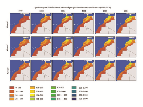
Figure 5 points out that the three groups of models captured the spatial distribution of precipitation pattern in Morocco, year by year. In general, northern Morocco is better watered than the south, and west is better watered than the east. The same figure helps to highlight the years that experienced relatively abundant rainfall (2001, 2003, and 2004) and the years that experienced low rainfall, such as 1999.
Although the estimated precipitation has captured the overall precipitation pattern over Morocco, some residual values were observed (Figure 6). Negative residual values indicate an underestimation of rainfall. This concerns the Saharan bioclimatic stage where vegetation is very sparse or absent, and hence vegetation growth is not proportional to the rainfall. The positive residual values indicate an overestimation of rainfall. This corresponds to the wettest areas of Morocco that is covered by forests and matorral, which are characterized by relatively deep roots and therefore do not have necessarily an immediate response to rainfall. Similar residual values were observed in Spain [10]. The final downscaled and calibrated precipitations for the six years according to Groups 2, 3, and 4 are presented in Figure 7.
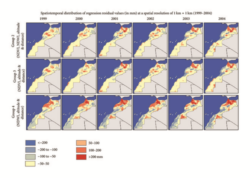
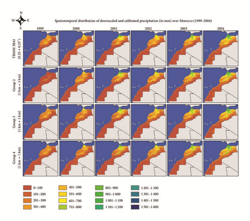
Figure 8 reports that all the correlation coefficients are important for the three groups. These coefficients range from 0,72 to 0,92 and are similar to or relatively higher than those found by other authors in China [11]. Also, model fittings have all passed the F statistical test (p < 0.001) and are statistically significant. This means that, in addition to having a finer spatial resolution of 1 km, the downscaled precipitation captured the pattern of TRMM 3B43.
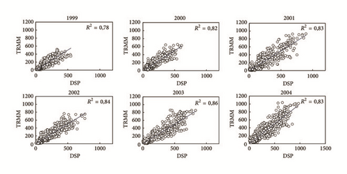
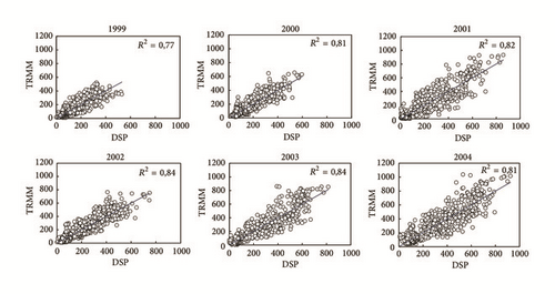
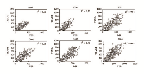
The higher values of R2 correspond to the models of Group 2 that range from 0.78 to 0.86, with an average of 0.83 for this group of models. The values of R2 of Group 3 are very close to those of Group 2. They range from 0.77 to 0.84, with an average of 0.81, while R2 of Group 4 is lower, with values ranging from 0.50 to 0.70 and an average of 0.61. Nevertheless, R2 of this last group remains important and statistically significant. The performance of the models of Group 2 could be explained by the fact that the models of this group include all variables. Aside from that, the models of Group 3 have good statistics compared to those of Group 4, since the models of Group 3 are based on NDVI, which is less dynamic than NDWI.
4.4. Validation of Downscaled and Calibrated Precipitation
Figure 9 reveals that the averages of R2 for the six years are 0.89, 0.87, and 0.79 for Groups 2, 3, and 4, respectively. The averages of these coefficients for the three groups are slightly lower than of the original TRMM 3B43. A similar result was observed by Duan and Bastiaanssen [1].
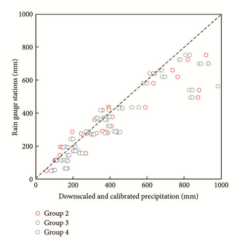
As mentioned earlier, the number of the used RGSs for spatial downscaling approach was 53, 61, 34, 34, 32, and 25 for the years 1999, 2000, 2001, 2002, 2003, and 2004, respectively (in function of data availability). In order to evaluate downscaled precipitation and to compare the models of Groups 2, 3, and 4, only independent rain gauge stations can be used. In this study, 10 available rain gauge stations were used to estimate the statistical metrics (R2, RMSE, MAE, and bias). It is worth mentioning that all downscaling studies cited earlier use independent rain gauge stations for the validation purpose.
According to Table 5, the RMSE values range from 26 to 167, from 20 to 158, and from 33 to 170 for Group 2, Group 3, and Group 4, respectively. In general, these values remain lower than those of TRMM 3B43. The bias is also more important for TRMM 3B43 compared to those of the three groups. Group 2 has lower bias (−0.021 to −0.006). The bias is between −0.026 and −0.06 and −0.027 and 0.037 for Group 3 and Group 4, respectively. The bias of Group 2 is systematically negative for the six years; this means that the downscaled precipitations of this group slightly underestimate the precipitation.
| 1999 | 2000 | 2001 | 2002 | 2003 | 2004 | ||
|---|---|---|---|---|---|---|---|
| R2 | TRMM | 0.98 | 0.95 | 0.89 | 0.98 | 0.76 | 0.84 |
| DSC Group 2 | 0.95 | 0.93 | 0.90 | 0.99 | 0.79 | 0.80 | |
| DSC Group 3 | 0.93 | 0.93 | 0.87 | 0.98 | 0.76 | 0.78 | |
| DSC Group 4 | 0.93 | 0.90 | 0.78 | 0.98 | 0.73 | 0.77 | |
| RMSE | TRMM | 24.91 | 64.24 | 143.41 | 68.22 | 107.33 | 180.46 |
| DSC Group 2 | 31.70 | 65.87 | 123.96 | 26.38 | 115.94 | 167.32 | |
| DSC Group 3 | 34.99 | 52.30 | 116.79 | 20.21 | 111.63 | 157.74 | |
| DSC Group 4 | 22.87 | 61.79 | 132.92 | 60.36 | 128.79 | 169.96 | |
| Bias | TRMM | 0.041 | 0.168 | 0.412 | 0.163 | 0.282 | 0.403 |
| DSC Group 2 | −0.014 | −0.013 | −0.017 | −0.006 | −0.006 | −0.021 | |
| DSC Group 3 | −0.017 | −0.021 | −0.018 | −0.006 | −0.007 | −0.028 | |
| DSC Group 4 | −0.020 | −0.027 | 0.037 | 0.016 | 0.015 | 0.036 | |
| MAE | TRMM | 20.171 | 56.524 | 95.229 | 46.494 | 64.107 | 119.856 |
| DSC Group 2 | 29.589 | 52.798 | 77.099 | 13.488 | 55.079 | 95.926 | |
| DSC Group 3 | 31.793 | 38.696 | 70.261 | 8.964 | 52.754 | 90.081 | |
| DSC Group 4 | 20.833 | 50.152 | 79.443 | 35.950 | 56.483 | 97.845 | |
It can be concluded that the models of Group 2, which were built using NDVI, NDWI, elevation, and distance, perform slightly better than the models of Groups 3 and 4. It is also evident that the models developed by stepwise regression based on NDWI, distance, and elevation have good agreement with the observed precipitation. However, these models perform slightly less than those of Group 3.
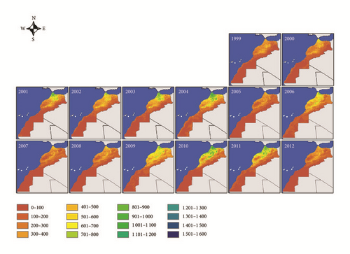
The developed methodology was applied to the recent years, from 2004 to 2012. This allowed us to have an updated picture of spatial distribution of precipitation over Morocco during the last 14 years at a spatial resolution of 1 km2 (Figure 10).
4.5. Limitations of the Downscaling Approach
4.5.1. Sensitivity to Bioclimatic Stages
The parameters of the regression models for the five bioclimatic stages are reported in Table 6. It seems that the subhumid stage is characterized by very high and significant R, with an average of 0.88 for the six years. The second area where the approach performs well is the semiarid stage, with an average of 0.8. The average R coefficient in the arid bioclimatic stage is around 0.65. The bioclimatic stages where R was lower are the humid and Saharan stages. In these stages, R ranged from 0.22 to 0.48 for the first and from 0.22 to 0.62 for the second.
| Years | Bioclimate | R2 | Max. VIF |
|---|---|---|---|
| 1999 | Humid | 0,10 | 2,91 |
| Subhumid | 0,80 | 2,03 | |
| Semiarid | 0,46 | 2,89 | |
| Arid | 0,42 | 2,64 | |
| Saharan | 0,37 | 2,81 | |
| 2000 | Humid | 0,08 | 5,89 |
| Subhumid | 0,87 | 1,06 | |
| Semiarid | 0,41 | 1,19 | |
| Arid | 0,38 | 1,15 | |
| Saharan | 0,31 | 1,57 | |
| 2001 | Humid | 0,09 | 4,61 |
| Subhumid | 0,62 | 1,08 | |
| Semiarid | 0,64 | 1,87 | |
| Arid | 0,33 | 1,00 | |
| Saharan | 0,05 | 1,00 | |
| 2002 | Humid | 0,07 | 3,42 |
| Subhumid | 0,71 | 1,00 | |
| Semiarid | 0,44 | 2,18 | |
| Arid | 0,51 | 2,70 | |
| Saharan | 0,39 | 2,57 | |
| 2003 | Humid | 0,23 | 7,56 |
| Subhumid | 0,83 | 1,11 | |
| Semiarid | 0,70 | 2,87 | |
| Arid | 0,57 | 1,54 | |
| Saharan | 0,22 | 1,15 | |
| 2004 | Humid | 0,05 | 5,36 |
| Subhumid | 0,82 | 1,21 | |
| Semiarid | 0,59 | 1,68 | |
| Arid | 0,30 | 1,48 | |
| Saharan | 0,24 | 1,69 | |
These low values of R in the Saharan bioclimatic stage can be explained by the nature of the vegetation cover in this area, which is very sparse or even nonexistent. It can also be due to the nature of soil, which is skeletal and sandy. Given these conditions, precipitation does not lead to a substantial growth of vegetation, since there are other limiting factors. Regarding the humid bioclimatic stage, low R could be explained by the coincidence of these areas with mountain peaks that are characterized by the presence of rocky outcrops and/or forests. Indeed, rocky outcrops are almost devoid of vegetation, while forests are characterized by deep roots that do not deplete the water needs directly and immediately from precipitation. It is worth mentioning that the low R in the Saharan bioclimatic stage could be affected also by the low number of RGSs. The same table reveals the absence of multicollinearity except in the humid stage where the maximum VIF value can reach 7.56.
4.5.2. Influence of Distance from the Mediterranean Sea
Among all the possible combinations of variables, for the five classes of distance over the six years, stepwise regression identified 74 statistically significant models, from which only 16 models include distance. This number is equal to 5, 4, 2, 0, and 5 for Classes 1, 2, 3, 4, and 5, respectively.
Figure 11 presents the average of standardized coefficients of the variable distance for the five classes. It appears that the absolute values of these coefficients are important for Class 1 and regress gradually for other classes.
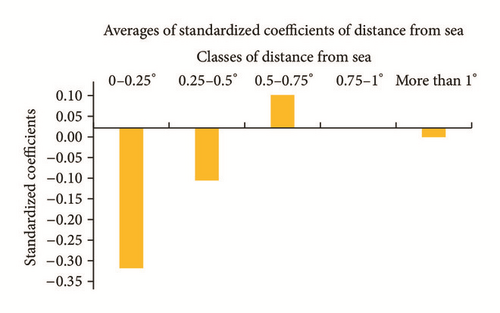
This result was confirmed through an ANOVA F-statistic test and was pursued further by applying Tamhane’s post hoc test, to verify whether there is a statistically significant difference between the standardized coefficients of pairwise classes. The result (Table 7) shows that there is a significant difference between Class 1 and Classes 3 and 5. The difference is small and not significant between Classes 1 and 2. There is a significant difference between Classes 2 and 5 and between Class 3 and Class 5.
| (A) Factor | (B) Factor | Mean difference (A − B) | Std. error | Sig. | 95% confidence interval | |
|---|---|---|---|---|---|---|
| Lower bound | Upper bound | |||||
| 0.00–0.25 | 0.25–0.50 | −0,19 | 0,0614264 | 0,165 | −0,458776 | 0,078376 |
| 0.50–0.75 | −0,37∗ | 0,0604362 | 0,015 | −0,650249 | −0,100151 | |
| More than 1° | −0,28∗ | 0,0694354 | 0,030 | −0,539721 | −0,028279 | |
| 0.25–0.50 | 0.00–0.25 | 0,19 | 0,0614264 | 0,165 | −0,078376 | 0,458776 |
| 0.50–0.75 | −0,18∗ | 0,0214165 | 0,008 | −0,293996 | −0,076004 | |
| More than 1° | −0,09 | 0,0403411 | 0,320 | −0,254147 | 0,066547 | |
| 0.50–0.75 | 0.00–0.25 | 0,37∗ | 0,0604362 | 0,015 | 0,100151 | 0,650249 |
| 0.25–0.50 | 0,18∗ | 0,0214165 | 0,008 | 0,076004 | 0,293996 | |
| More than 1° | 0,09 | 0,0388167 | 0,345 | −0,076030 | 0,258430 | |
| More than 1° | 0.00–0.25 | 0,28∗ | 0,0694354 | 0,030 | 0,028279 | 0,539721 |
| 0.25–0.50 | 0,09 | 0,0403411 | 0,320 | −0,066547 | 0,254147 | |
| 0.50–0.75 | −0,09 | 0,0388167 | 0,345 | −0,258430 | 0,076030 | |
- ∗The mean difference is significant at the 0.05 level.
According to this analysis, it was seen that the standardized coefficients of the variable distance are larger in Classes 1 and 2 than in Classes 3 and 4. It can be concluded that the predictor distance has a relatively large and statistically significant contribution in Classes 1 and 2. The contribution of this variable over Classes 3 and 4 is nonsignificant. It is the same for Class 5 since the unstandardized coefficients are very small, with an average of −0.02.
5. Conclusion
This study investigated the spatial downscaling of coarse satellite-derived precipitation over five bioclimatic stages in Morocco, for a period of 14 years, from 1999 to 2012. The case of TRMM 3B43 was studied through multiple stepwise regressions and AIC based on an open dataset including NDVI, NDWI, elevation, and distance from sea.
The study demonstrated the existence of a strong and statistically significant relationship between NDVI and TRMM 3B43, with correlation coefficients reaching 0.81. The integration of the predictors elevation and distance from sea in these regression models can slightly improve the correlation coefficients,. Likewise, the standardized coefficients of NDWI are high and statistically significant, meaning that they have a high contribution to the selected models.
The pairwise comparisons of the selected models through stepwise regression and AIC with those based on multiple regression showed that the first ones are more performant than the second. In fact, the stepwise regression and AIC allowed refining more the models by choosing the best combination of predictors and therefore the most robust and significant models (best-fit models).
The findings allowed concluding that both NDVI and NDWI based regression models have significant regression parameters and they can be used to downscale TRMM precipitation. However, the statistical parameters of the regression models based on NDVI present better performance. The statistical metrics for this group can reach 0.99 for R2, 26.38 for RMSE, −0.006 for bias, and 13.48 for MAE.
The downscaled precipitation at 1 km captured the overall spatiotemporal precipitation pattern of Morocco. The results showed a good agreement with RGS measurements. It is worth mentioning that the stepwise regression models built using the four predictors present the best agreement and therefore the best approximation of precipitation at a spatial resolution of 1 km for the six years.
The analysis of the influence and the contribution of distance from sea showed that the most significant correlations were noted in the first and second classes that spread over a distance of 0.50° (54 km approximately). Beyond this threshold, the predictor (distance from sea) does not have any significant contribution.
The study demonstrated the highest performance of the spatial downscaling approach in the subhumid, semiarid stages and in the arid bioclimatic stages, to a lesser extent. The coefficients of determination noted in these areas can reach up to 0.87, 0.70, and 0.57, respectively. However, the proposed approach seems sensitive and therefore not adapted to the relatively extreme climatic conditions, such as the Sahara and humid stages, given the very low correlation coefficients obtained based on the stepwise regression in these stages.
Conflicts of Interest
The authors declare that there are no conflicts of interest regarding the publication of this article.
Acknowledgments
The authors would like to acknowledge the support of the IRIACC Initiative and specifically IDRC-Canada for the sponsorship of the project entitled “Faire-Face aux Changements Ensemble: Mieuxs’adapter aux Changements Climatiques au Canada et en Afrique de l’Ouest” (Project no. 106372-013).


