Option Price Decomposition in Spot-Dependent Volatility Models and Some Applications
Abstract
We obtain a Hull and White type option price decomposition for a general local volatility model. We apply the obtained formula to CEV model. As an application we give an approximated closed formula for the call option price under a CEV model and an approximated short term implied volatility surface. These approximated formulas are used to estimate model parameters. Numerical comparison is performed for our new method with exact and approximated formulas existing in the literature.
1. Introduction
In [1], a decomposition of the price of a plain vanilla call under the Heston model is obtained using Itô calculus. Recently, in [2], the decomposition obtained in [1] has been used to infer a closed form approximation formula for a plain vanilla call price in the Heston case, and on the basis of this approximated price, a method to calibrate model parameters has been developed and successfully applied. In this paper, we use the ideas presented in [1] to obtain a closed form approximation to plain vanilla call option price under a spot-dependent volatility model.
The model presented here assumes the volatility is a deterministic function of the underlying stock price, and therefore, there is only one source of randomness in the model. These models are sometimes called local volatility models in the industry and GARCH-type volatility models in financial econometrics. Recall that these models are different from the so-called stochastic volatility models, like Heston model, where the volatility process is driven by an additional source of randomness, not perfectly correlated with the stock price innovations.
As an application, for the particular case of CEV model, we obtain an approximation of the at-the-money (ATM) implied volatility curve as a function of time and an approximation of the implied volatility smile as a function of the log-moneyness, close to the expiry date. We use these approximations to calibrate the CEV model parameters.
2. Preliminaries and Notations
- (i)
We define the Black-Scholes function as a function of t ∈ [0, T] and x, y ∈ [0, ∞) such that
() -
where Φ(·) denotes the cumulative probability function of the standard normal law, K and T are strictly positive constants, and
() -
Note that the price of a plain vanilla European call under the classical Black-Scholes theory is BS(t, St, σ) where St is the price of the underlying process at t, σ is the constant volatility, K is the strike price, and T is the expiry date.
- (ii)
We will denote frequently by τ≔T − t the time to maturity.
- (iii)
We use in all the paper the notation , where is the completed natural filtration of S.
- (iv)
In our setting, the call option price is given by
() - (v)
Recall that from the Feynman-Kac formula, the operator
() -
satisfies .
- (vi)
We define the operators Λ≔x∂x, , and Γ2 = Γ∘Γ. In particular, we have that
()
Lemma 1. Then, for any n ≥ 2, and for any positive quantities x, y, p, and q, one has
Proof. For any n ≥ 2 we have
3. A General Decomposition Formula
Here we obtain a general abstract decomposition formula for a certain family of functionals of S that will be the basis of all later computations.
Then we have the following lemma.
Lemma 2 (generic decomposition formula). For all t ∈ [0, T], one has
Proof. Applying the Itô formula to process e−rtA(t, St, θ2(St))B(t) we obtain
Now, applying Feynman-Kac formula for , multiplying by ert, and taking conditional expectations, we obtain
On the other hand, using Itô calculus rules, it is easy to see that
Finally, substituting this expression in (12) we finish the proof.
For the Black-Scholes function previous lemma reduces to the following corollary.
Corollary 3 (BS decomposition formula). For all t ∈ [0, T], one has
Proof. Applying Lemma 2 to A(t, St, θ2(St))≔BS(t, St, θ(St)) and B(t) ≡ 1, and using equalities
Remark 4. For clarity, in the following we will refer to terms of the previous decomposition as
Remark 5. In [4], an alternative formula that can be used for local volatility models is proved. The formula presented in [4] uses, as a base function, function BS(t, St, σ), but this formula is numerically worse than the new formula presented here that uses as a base function BS(t, St, θ(St)). This happens because in the formula presented in [4] the volatility is put into the approximated term, instead of keeping it on the Black-Scholes term as we do here. It is precisely because volatility is a deterministic function of the underlying asset price that we can do that.
4. Approximation Formula
In this section we obtain an approximation formula to plain vanilla call price by approximating terms (I)–(IV). The main idea is to use again Lemma 2 to estimate the errors.
Theorem 6 (BS decomposition formula with error term). For all t ∈ [0, T], one has
Proof. We apply Lemma 2 to terms (I)–(IV). Concretely, functions A and B in every case are
(I)
(II)
(III)
(IV)
5. CEV Model
There exists a closed form formula for call options; see [5, 6]. An approximated formula is given in [7].
5.1. Approximation of the CEV Model
Applying Corollary 3 to CEV model, we obtain the following.
Corollary 7 (CEV exact formula). For all t ∈ [0, T], one has
The exact formula can be difficult to use in practice, so we will use the following approximation.
Corollary 8 (CEV approximation formula). For all t ∈ [0, T], one has
5.2. Numerical Analysis of the Approximation for the CEV Case
The results for a call option with parameters β = 0.25, S0 = 100, K = 100, σ = 20%, and r = 1% are presented in Table 1.
| Parameters | Exact formula | Approximation | HW | ||
|---|---|---|---|---|---|
| T − t | Price | Price | Error | Price | Error |
| 0.25 | 0.2882882 | 0.2882884 | −1.92E − 07 | 0.2882019 | 8.64E − 05 |
| 1 | 1.0103060 | 1.0103070 | −9.78E − 07 | 1.0100377 | 2.68E − 04 |
| 2.5 | 2.4709883 | 2.4709894 | −1.04E − 06 | 2.4708310 | 1.57E − 04 |
| 5 | 4.8771276 | 4.8771278 | −2.22E − 07 | 4.8771099 | 1.77E − 05 |
The results in the case that β = 0.50 are presented in Table 2.
| Parameters | Exact formula | Approximation | HW | ||
|---|---|---|---|---|---|
| T − t | Price | Price | Error | Price | Error |
| 0.25 | 0.5356736 | 0.5356765 | − 2.89E − 06 | 0.5354323 | 2.41E − 04 |
| 1 | 1.3886303 | 1.3886529 | − 2.26E − 05 | 1.3868801 | 1.75E − 03 |
| 2.5 | 2.8506826 | 2.8507669 | − 8.42E − 05 | 2.8450032 | 5.68E − 03 |
| 5 | 5.1658348 | 5.1660433 | − 2.09E − 04 | 5.1543092 | 1.15E − 02 |
The results in the case that β = 0.75 are presented in Table 3.
| Parameters | Exact formula | Approximation | HW | ||
|---|---|---|---|---|---|
| T − t | Price | Price | Error | Price | Error |
| 0.25 | 1.3887209 | 1.3887438 | − 2.30E − 05 | 1.3883284 | 3.92E − 04 |
| 1 | 3.0389972 | 3.0391797 | − 1.83E − 04 | 3.0359001 | 3.10E − 03 |
| 2.5 | 5.2954739 | 5.2961870 | − 7.13E − 04 | 5.2835621 | 1.19E − 02 |
| 5 | 8.2781049 | 8.2800813 | − 1.98E − 03 | 8.2459195 | 3.22E − 02 |
Finally, the results in the case that β = 0.90 are presented in Table 4.
| Parameters | Exact formula | Approximation | HW | ||
|---|---|---|---|---|---|
| T − t | Price | Price | Error | Price | Error |
| 0.25 | 2.6404164 | 2.6404455 | − 2.92E − 05 | 2.6401025 | 3.14E − 04 |
| 1 | 5.5191736 | 5.5194053 | − 2.32E − 04 | 5.5166821 | 2.49E − 03 |
| 2.5 | 9.1446125 | 9.1455159 | − 9.03E − 04 | 9.1349142 | 9.70E − 03 |
| 5 | 13.5553379 | 13.5578351 | − 2.50E − 03 | 13.5286009 | 2.67E − 02 |
Note that the new approximation is more accurate than the approximation obtained in [7].
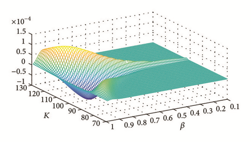
In Figure 1, we plot the surface of errors between the exact formula and our approximation.

We calculate also the speed time of execution (in seconds) of every method running the function timeit of Matlab 1.000 times. The computer used is an Intel Core i7 CPU Q740 @1.73 GHz 1.73 GHz with 4 GB of RAM with a Windows 10 (×64). The results are presented in Table 5.
| Measure | Exact formula | Approximation | HW |
|---|---|---|---|
| Average | 2.56E − 02 | 1.73E − 04 | 1.67E − 04 |
| Standard deviation | 3.03E − 03 | 2.86E − 05 | 2.52E − 05 |
| Max | 4.68E − 02 | 3.65E − 04 | 3.67E − 04 |
| Min | 2.42E − 02 | 1.64E − 04 | 1.59E − 04 |
We observe that singular perturbation method is the fastest method to calculate the price of CEV call option. The method developed in this work is a little more expensive in computation time. But to compute the exact price is much more expensive than any of the other two methods. Note that, in our method, we also are able to calculate at the same time the price and the Gamma of the log-normal price.
6. The Approximated Implied Volatility Surface under CEV Model
In the above section we have computed a bound for the error between the exact and the approximated pricing formulas for the CEV model. Now, we are going to derive an approximated implied volatility surface of second order in the log-moneyness. This approximated implied volatility surface can help us to understand better the volatility dynamics. Moreover we obtain an approximation of the ATM implied volatility dynamics.
6.1. Deriving an Approximated Implied Volatility Surface for the CEV Model
Note that I1(T, K) is linear with respect to the log-moneyness, while I2(T, K) is quadratic.
Remark 9. Note that the pricing formula has an error of O((β − 1) 2) as we have proved in Corollary 8, and this is translated into an error of O((β − 1) 2) into our approximation of the implied volatility. The quadratic term of the volatility shape is not accurate.
We calculate now the short time behavior of the approximated implied volatility . We write the approximated equations in terms of 1 − β, because the case β < 1 is the most interesting, and in terms of the log-moneyness lnK − lnS0.
Lemma 10. For T close to 0 one has
Proof. Note that
Remark 11. Note that (34) is a parabolic equation in the log-moneyness. Also, from the above expression it is easy to see that the slope with respect to lnK is negative when K < S0exp(3/2(1 − β)) and positive when K > S0exp(3/2(1 − β)), showing that the implied volatility for short times to maturity is smile-shaped. This is consistent with the result in [11]. Furthermore, there is a minimum of the implied volatility with respect to lnK attained at K = S0exp(3/2(1 − β)).
Remark 12. Note that, in stochastic volatility models, the implied volatility depends homogeneously on the pair (S, K), and in fact it is a function of the log-moneyness ln(S0/K). As extensively discussed in [12] and exemplified for GARCH option pricing in [13], this homogeneity property is at odds with any type of GARCH option pricing. We found also this phenomenon in the quadratic expansion (34).
6.2. Numerical Analysis of the Approximation of the Implied Volatility for the CEV Case
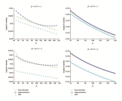
In Figure 2, we can see that the implied volatility dynamics behaves well for long dated maturities and short dated maturities when β is close to 1. When this is not the case, the formula behaves well at-the-money but the error increases far from the ATM value. This behavior is a consequence of the quadratic error of our approximation.

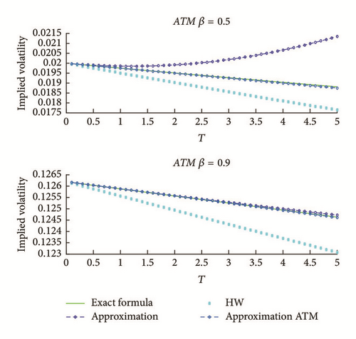
Comparing the ATM volatility structure, we have the following graphics.
In Figure 3, we observe that, for ATM options, the approximated implied volatility surface fits really well the real implied volatility structure.

Now, we put the implied volatility approximation found in (34) into Black-Scholes formula and compare the obtained results with Hagan and Woodward results. The results for a call option with parameters β = 0.25, S0 = 100, K = 100, σ = 20%, and r = 1% are presented in Table 6.
| Parameters | Exact formula | BS with implied volatility (34) | HW | ||
|---|---|---|---|---|---|
| T | Price | Price | Error | Price | Error |
| 0.25 | 0.2882882 | 0.2882882 | 3.51E − 08 | 0.28820185 | 8.64E − 05 |
| 1 | 1.0103060 | 1.0103057 | 2.36E − 07 | 1.010037675 | 2.68E − 04 |
| 2.5 | 2.4709883 | 2.4709880 | 2.94E − 07 | 2.470830954 | 1.57E − 04 |
| 5 | 4.8771276 | 4.8771275 | 6.72E − 08 | 4.877109923 | 1.77E − 05 |
The results in the case that β = 0.50 are presented in Table 7.
| Parameters | Exact formula | BS with implied volatility (34) | HW | ||
|---|---|---|---|---|---|
| T | Price | Price | Error | Price | Error |
| 0.25 | 0.5356736 | 0.5356732 | 4.27E − 07 | 0.53543231 | 2.41E − 04 |
| 1 | 1.3886303 | 1.3886267 | 3.65E − 06 | 1.386880117 | 1.75E − 03 |
| 2.5 | 2.8506826 | 2.8506672 | 1.54E − 05 | 2.845003212 | 5.68E − 03 |
| 5 | 5.1658348 | 5.1657911 | 4.36E − 05 | 5.154309238 | 1.15E − 02 |
The results in the case that β = 0.75 are presented in Table 8.
| Parameters | Exact formula | BS with implied volatility (34) | HW | ||
|---|---|---|---|---|---|
| T | Price | Price | Error | Price | Error |
| 0.25 | 1.3887209 | 1.3887176 | 3.29E − 06 | 1.388328423 | 3.92E − 04 |
| 1 | 3.0389972 | 3.0389707 | 2.64E − 05 | 3.035900123 | 3.10E − 03 |
| 2.5 | 5.2954739 | 5.2953686 | 1.05E − 04 | 5.283562121 | 1.19E − 02 |
| 5 | 8.2781049 | 8.2778040 | 3.01E − 04 | 8.245919491 | 3.22E − 02 |
And the results in the case that β = 0.90 are presented in Table 9.
| Parameters | Exact formula | BS with implied volatility (34) | HW | ||
|---|---|---|---|---|---|
| T | Price | Price | Error | Price | Error |
| 0.25 | 2.6404164 | 2.6404122 | 4.17E − 06 | 2.640102524 | 3.14E − 04 |
| 1 | 5.5191736 | 5.5191404 | 3.31E − 05 | 5.51668209 | 2.49E − 03 |
| 2.5 | 9.1446125 | 9.1444830 | 1.29E − 04 | 9.134914233 | 9.70E − 03 |
| 5 | 13.5553379 | 13.5549787 | 3.59E − 04 | 13.52860091 | 2.67E − 02 |
Our approximation is better than Hagan and Woodward one.
We compare also execution times (see Table 10).
| Measure | HW | BS with implied volatility (34) |
|---|---|---|
| Average | 1.67E − 04 | 1.66E − 04 |
| Standard deviation | 2.52E − 05 | 2.37E − 05 |
| Max | 3.67E − 04 | 3.48E − 04 |
| Min | 1.59E − 04 | 1.58E − 04 |
We can observe that both formulas are similar in computation time, with the new approximation formula being a bit faster.
6.3. Calibration of the Model
Following the ideas of [2], we propose a method to calibrate the model. This method will allow us to find σ and β using quadratic linear regression. We can recover the parameters with a set of options of the same maturity with (34) or with ATM options of different maturities (36).
6.3.1. Calibration Using the Smile of Volatility
6.3.2. Calibration Using ATM Implied Volatilities
We have seen that to do a quadratic regression is enough to recover a good approximation of the parameters.
7. Conclusion
In this paper, we notice that ideas developed in [1] for Heston model can be used for spot-dependent volatility models. It is interesting to realize that the approximation found in this case has more terms than the one obtained for stochastic volatility models (see [4]). We have applied this technique to the CEV model, doing a comparison between exact prices, Black-Scholes using Hagan and Woodward implied volatility, and our price approximation. We have seen that our approximation is better than Hagan and Woodward approximation for pricing, but a bit more expensive in computation time. As well, we have calculated an approximation of the implied volatility as the limit of the implied volatility close to zero as a function of log-moneyness and an approximation of the ATM implied volatility as a function of time. We have compared our approximation with the exact implied volatility and Hagan and Woodward approximation. We note that if we put our implied volatility approximation into Black-Scholes function, we get a better approximation than Hagan and Woodward in the same computation time. So we have developed an easy way to calibrate CEV model that consists essentially in doing a quadratic regression.
Conflicts of Interest
The authors declare that there are no conflicts of interest regarding the publication of this article.
Acknowledgments
Josep Vives was partially supported by Grant MEC MTM 2013 40782 P.
Appendix
In the following appendices we obtain the error terms of the decomposition in Theorem 6 (Appendix A), the same formulas in the particular case of CEV model (Appendix B), and upper-bounds for those terms using Lemma 1 (Appendix C). In all the section we write τu≔T − u.
A. Decomposition Formulas in the General Model
A.1. Decomposition of Term (I)
A.2. Decomposition of Term (II)
A.3. Decomposition of Term (III)
A.4. Decomposition of Term (IV)
B. Decomposition Formulas for the CEV Model
B.1. Decomposition of the Term (ICEV)
B.2. Decomposition of the Term (IICEV)
B.3. Decomposition of the Term (IIICEV)


