A BP (backpropagation) neural network method is employed to solve the problems existing in the synthetic characteristic curve processing of hydroturbine at present that most studies are only concerned with data in the high efficiency and large guide vane opening area, which can hardly meet the research requirements of transition process especially in large fluctuation situation. The principle of the proposed method is to convert the nonlinear characteristics of turbine to torque and flow characteristics, which can be used for real-time simulation directly based on neural network. Results show that obtained sample data can be extended successfully to cover working areas wider under different operation conditions. Another major contribution of this paper is the resampling technique proposed in the paper to overcome the limitation to sample period simulation. In addition, a detailed analysis for improvements of iteration convergence of the pressure loop is proposed, leading to a better iterative convergence during the head pressure calculation. Actual applications verify that methods proposed in this paper have better simulation results which are closer to the field and provide a new perspective for hydroturbine synthetic characteristic curve fitting and modeling.

1. Introduction

Many hydropower plants have been built worldwide to harness the energy of falling or running water for electricity purpose [1, 2]. A lot of fruitful and meaningful works of hydropower turbine in advanced control [3–6], parameter identification [7–9], dynamics analysis [10, 11], and fault diagnosis [12] have been done. In addition, obtaining of flow and torque characteristics from synthetic characteristic curve of a specific Francis turbine is the key to high-precision nonlinear simulation and stability analysis [13], which could serve to maintain safe, stable, and economical operation of hydropower generating unit. Thus, it is extremely important for hydroturbine governing system nonlinear modeling and control [4, 8, 11, 14] to process the synthetic characteristic curve in a reasonable way. However, synthetic characteristic curves that provided by manufacturers nowadays are only in the high efficiency and large guide vane opening area in China, which is far from meeting the research requirements of transition process, especially in large fluctuations. So it is necessary to extend and complement the synthetic characteristic curves for further research. In view of this, many scholars have carried out a lot of studies on this problem. For example, a radial basis function neural network method was used in [15] for data processing of hydroturbine synthetic characteristic curve; the discrete sample data obtained from synthetic characteristic curve were fitted effectively. Moreover, data in unknown region could be predicted successfully by combining the boundary constraint conditions. However, the radial basis function neural network can be affected by the dispersion constant easily, and there is no specific method for the selection of the dispersion constant, which can only be chosen tentatively in [13]. Discontinuity of derivative in interpolation method for hydroturbine modeling was solved to improve the iterative convergence of head pressure calculation with BP neural network in [16]; irregular discrete sample data were processed quite well with the Delaunay triangulation algorithm in [17]. But none of the works stated above [13–17] can solve the problem of acquiring characteristic data in the nonhigh efficient areas. Besides, literature review shows that many other methods, such as the artificial experience, approximate linear interpolation, spline interpolation, table interpolation, and shape function interpolation, have also been applied to the characteristics processing of hydroturbine, but all these methods have their own limitations. Motivated by this, a special method based on BP neural network is proposed in the paper for Francis turbine modeling and real-time simulation, the proposed method consists of various steps as follows: (1) extract multisets of sample data, which can comprehensively represent the characteristics of the turbine and meet the requirements of the transition process, then normalize and store these sample data in the text file in standard form; (2) extend the characteristic curve to unknown low efficiency area, such as small guide vane opening and small unit speed area, based on the acquired sample data and boundary constraint; (3) train the extended sample data with neural network and save the obtained weight and threshold value in forms of text for calling. In addition, a detailed analysis for improvements of traditional simulation algorithm is given: the discrete systems resampling technique is proposed to overcome the limitation of sampling period contradiction existing between diversion system and hydroturbine governing system; a different mathematical method based on the neural network surface is illustrated to improve the iterative convergence of head pressure in simulation.

The rest of the paper is outlined as follows: in Section 2, synthetic characteristic curve processing method of Francis turbine and an example application are presented in detail. Resampling technology based on characteristic line is constructed in Section 3. Investigations on improving convergence of head pressure loop are shown in Section 4. Section 5 illustrates the simulation results along with discussions and remark words. Conclusions are provided in Section 6.

2. Synthetic Characteristic Curve Processing Method of Francis Turbine

Obtaining the description that expresses the relationship between flow and torque characteristics through model synthetic characteristic curve is the most common method for hydroturbine nonlinear modeling. The main idea is to store the processed discrete sample data, which comes from model synthetic characteristic curve, in a certain way (array of expressing surfaces, neural network, etc.) in advance; then flow and torque characteristics can be calculated by interpolation or neural network method according to the change of operating condition.

It is no longer required to establish the specific expression function when extending and fitting sample data through neural network. Besides, sample data in unknown region can be predicted to improve the working efficiency and data processing accuracy of synthetic characteristic curve by combining with the boundary constraints.

A general method for flow and torque characterization with BP neural network is discussed here. Firstly, access and extension steps of sample data are given from the perspective of the model synthetic characteristic curve and runaway characteristics curve; then forms and structures of neural network are determined based on the analysis and comparison; in the end, the neural network is trained offline with the Matlab neural network toolbox for real-time simulation modeling.

2.1. Reading, Processing, and Extension of Sample Data

Access to sample data refers to the obtaining process of flow, efficiency, and runaway characteristics from model synthetic and runaway characteristics curve. Sample data processing is the calculation for torque characteristics through obtained flow and efficiency characteristics sample data. In most cases, the model synthetic characteristic curve provided is only within the high efficiency area, which is far from enough for nonlinear real-time modeling and simulation. Thus, prior knowledge and known information method to expand the sample data, namely extension, is used in the paper. Flow chart of data process steps from (a) to (f) is given in Figure 1.

Details are in the caption following the image — **Figure 1**
Open in figure viewer PowerPoint

Flow chart of sample data reading, processing, and extension.

(a) Reading Flow Characteristics. The flow characteristic is obtained by reading a certain number of data points at each equal opening degree line on model synthetic characteristic curve:

()

where a_i, N_11i, Q_11i are vane opening, unit speed, and unit flow, respectively. Quantity and location of the data points are not defined strictly and can be determined according to the accuracy requirement of the object. More points and time are required to train the neural network when a higher accuracy is required. All of these data points in (1) can be used as sample data for flow characteristics.

(b) Reading Efficiency Characteristics. Conventional method can be used directly to obtain torque characteristics, which can also be carried out by reading the efficiency data point. Considering that the interspacing between different efficiency lines is generally large, which is conducive to data reading and reflect torque characteristics more comprehensively, the second method is employed in this study. A certain number of data points are read on each equal efficiency line η from model synthetic characteristic curve:

()

(c) Reading Runaway Characteristics. Read a certain number of data points on the runaway curve:

()

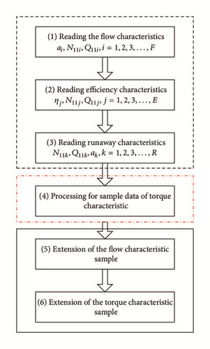
Value of a_k is selected to be identical to that of a_i in flow characteristics sample data for convenience.

(d) Processing for Sample Data of Torque Characteristic. The numerical method can be got with proper fitting methods such as polynomial based higher order surface fitting or neural network fitting, through the obtained efficiency characteristics sample data:

()

Calculating η_i by N_11i, Q_11i of flow characteristics sample data and then unit torque M₁₁ can be carried out by the following formula:

()

where M₁₁, Q₁₁, N₁₁ and η are the unit torque (kN·m), unit flow (m³/s), unit speed (r/min) and efficiency, respectively. Then M_11i, N_11i, and a_i, i = 1,2, 3, …, F constitute the sample data of torque characteristics.

(e) Extension of the Flow Characteristic Sample. It is worth pointing out that flow characteristics with runaway speed are contained in turbine model runaway characteristic itself. Therefore, all the sample data in (3) can be added to the flow characteristics sample data (1). In addition, when the guide vane opening a = 0, and turbine flow will be zero regardless of speed, which helps to construct boundary conditions as follows:

()

where N₁₁₁, N₁₁₂, …, N_11N are N points that distributed arbitrarily between zero and the maximum unit speed. Finally, the new flow sample data can be obtained by incorporating sample data (6) into the sample (1):

()

(f) Extension of the Torque Characteristic Sample. Boundary conditions of torque characteristics of hydroturbine at zero opening are firstly added for extension. In this case, relationship between torque and speed is given as follows:

()

Here, K is normal numbers given in advance. Torque sample data are constructed at zero opening by following equation:

()

where N₁₁₁, N₁₁₂, …, N_11n are P points distributed arbitrarily between zero unit speed and the maximum possible.

What is more, when the turbine operates in the runaway condition, output torque is zero, so N_11k and M_11k, k = 1,2, 3, …, R corresponding to a_k, can be used as sample data of torque characteristic directly. Incorporating this sample data and (9) into the torque characteristic sample calculated by (5), then the new extended torque sample N_11m, a_m and M_11m, m = 1,2, 3, …, F + R + P can be obtained.

2.2. Selection of Neural Network

In spite of the sample data extension, neither the flow nor the torque characteristics sample data could cover all possible operating conditions of turbines. It is natural to solve the problem by training the flow and torque neural networks with obtained sample data above, then estimating the flow and torque characteristics in these unknown regions by a smooth extension with well-trained neural networks.

Using artificial neural network to realize the nonlinear characteristic of hydroturbine has the advantages of less data quantity, simpler calculation, controllable precision, and continuous derivative. Considering that this extension is polynomial fitting actually, available networks are mainly the BP neural network and the RBF neural network. Compared with RBF neural network, BP neural network has the following advantages.

(1) Structure of BP neural network is much simpler with the same approximation accuracy. In addition, the number of hidden layer neurons of RBF network is much higher than that of BP network when the sample data is increased, which makes the RBF network more complex in structure, leading to higher computational demand;

(2) There is a high degree of self-learning and adaptive ability and can extract the data association from input and output data automatically; moreover, learning content is stored in the weights of network adaptively.

(3) BP neural network will not have great impact on the global training results after suffering damage to the local or partial neurons. The system has a certain fault tolerance and can work normally when local damage happens.

The suitable neural network structure is selected for sample data training by comparing the number of neurons, time consuming of network training, amount of computation, training accuracy, and the controllability of training process.

2.3. BP Neural Network Training

The sample data are divided into training and validation data set randomly: 80% of the data are used to train the neural network, and the remaining 20% are used to verify the effect of neural network training. A loop control is set up in training process, so that the sample can be trained to find the optimal training results and final output is saved in forms of text.

2.4. Application Examples

A Francis turbine HLA339-LJ-450 with the rated head 176 m, rated power 225 MW, rated speed 200 r/min, and rated flow 142.5 m³/s, respectively, is used as an example in this study.

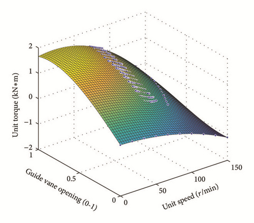
There are 716 sets of sample data obtained from synthetic characteristic curve in total, including 219 sets of flow characteristic sample data, 479 sets of efficiency characteristic sample data, and 18 sets of runaway characteristic sample data. Obtained sample data is extended based on the aforementioned 4 boundary conditions, and fitting surfaces of these samples are shown in Figures 2 and 3: points in the middle section of the diagrams are flow and its corresponded torque characteristic sample data; points in the right rear section of the diagrams are extended runaway flow and extended runaway torque characteristics sample data; points in the right front section of the diagrams are extended flow and its corresponded torque characteristic sample data with zero opening. It can be seen that even the extended sample data are failed to cover all possible operating conditions of the turbine and further training by neural network is needed.

The available networks are BP and RBF neural network. Only difference between the two networks is the calculating method of neurons. Computational demands of these two networks are in the same order with the same number of neurons and structure. When using BP neural network toolbox as a training tool, training time is longer; and results of each training may have a big difference because of the difference in initial value of each weight and the threshold. So it is necessary to choose the better results by human intervention. RBF network behaves better in this regard; however, it is necessary to specify the value of a distribution constant spread before training, which is closely related to the accuracy of the training. Therefore, the training is a process of repeated testing. What is more, accuracy of BP network is better than that of RBF network structure with the same network structure in general. This also means that RBF network requires more neurons and a larger amount of computation with the same approximation accuracy compared to BP network. Based on a large number of experiments and analyses above, a multilayer BP network with typical double input, single output, and five neurons is used to perform the nonlinear calculation for flow and torque characteristics. Structure of BP network is shown in Figure 4.

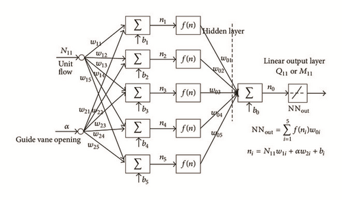
This is a typical double input, single output double BP network that includes five neurons. The standard log-sigmoid function is chosen as transfer function of hidden layer neurons here, which can be expressed as

()

Corresponding algorithm of neural network in Figure 4 can be expressed as follows:

()

Specific steps of sample data training with BP network structure are as follows.

Firstly, BP neural network net = newff(minmax(p), [5 1], {＇logsig＇＇purelin＇}) (where p is the input value of training sample data, which is a two-dimensional array that consists of the guide vane opening and unit flow in this case) is employed.

Secondly, the training parameters are set as follows:

net.trainParam.epochs = 1000
net.trainParam.goal = 0.00001
net.trainParam.min_grad = 1.0000e − 015

Thirdly, [net,tr]=train(net,trainV.P,trainV.T,[],[]) function is used for network training.

Finally, use network a = sim (net, p2) for simulation.

Finally, the output weight and threshold parameter of flow neural network and torque neural network are stored in the data file for turbine characteristics fitting.

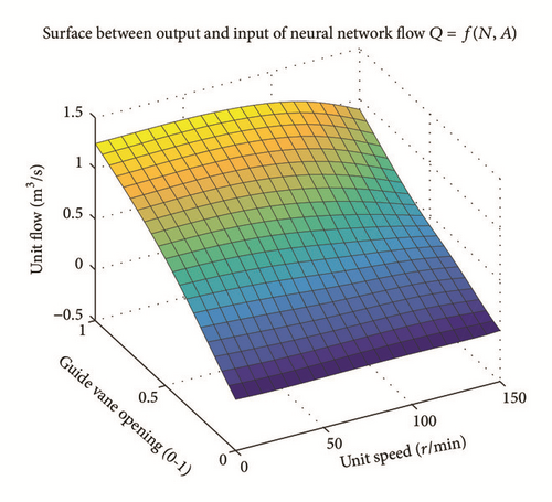
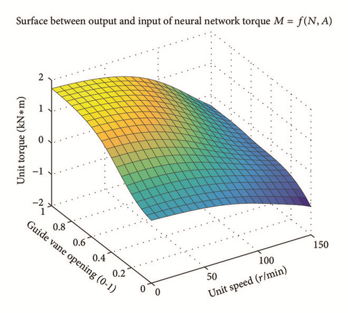
Relationship between flow and torque characteristics can be obtained by network fitting and training with extended flow and torque sample data, as shown in Figures 5 and 6. Compared with preliminary fitting surface in Figures 2 and 3, many known condition points are added to sample data manually according to actual situation of artificial experience based on the aforementioned extension sample data. The fitting error and control precision are set in training to ensure the smooth of surface from large vane opening to a small vane opening in transition. Working areas are covered more widely and a more comprehensive reflection of the turbine under different operation conditions is obtained.

2.5. Result Analysis

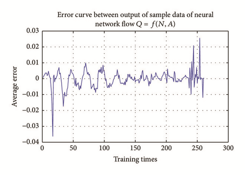
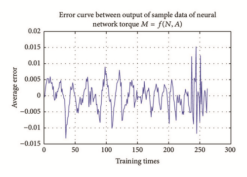
Fitting errors of flow and torque network are shown in Figures 7 and 8. The error can be controlled within ±0.04 and ±0.02, respectively, after training, which can reflect the real characteristics of the turbine in different operating conditions. Many causes may lead to the errors, such as error produced in the process of synthesis characteristic curve drawing, reading and fitting error in neural network training. For the third one, errors can be solved by increasing the number of hidden layer neurons to improve the approximation accuracy. In general, network’s ability of approximation accuracy is stronger with more neurons. But if the error is caused by the discrete characteristic of the data, there is no advantage to increase the number of neurons. On the contrary, it may affect the smoothness of surface sometimes and has certain impact on the convergence of simulation algorithm. Therefore, influence of various factors on the nonlinear characteristics should be fully considered to meet the requirements of hydropower units in real-time simulation when using neural network for training.

2.6. Brief Summary of Synthetic Characteristic Curve Processing Method

Design method for synthetic characteristic curve processing of Francis turbine can be summarized as follows: firstly, sample data obtained from the synthetic characteristic curve is normalized as standard format within [−1, +1] with mapminmax() function, which can help the neural network learn and train; then, extend the sample data mainly based on the following 4 boundary conditions [13].

(1) Boundary of runaway characteristics curve: when the unit operates in the runaway condition, its efficiency and torque are zero, and relationship among unit flow Q₁₁, unit speed N₁₁ vane opening, and a can be obtained according to Q ~ a and N ~ a curve from runaway curve.

(2) When the guide vane opening and unit speed are zero, the unit flow and unit torque are zero too;

(3) When the guide vane opening is zero, unit flow of turbine will be zero regardless of unit speed. At this time, ployfit() function can be used for polynomial fitting to carry out the unit torque M₁₁ that corresponds to different guide vane opening a with each fixed unit speed n. Then use ployval() function to get the corresponding unit torque under the fixed unit speed when the gate opening a = 0. Unit torque with different unit speed at a = 0 can be got by this way. Usually, M₁₁ < 0 when a = 0, and the relationship between M₁₁ and n₁₁ will meet the equation approximately, where k is the constant coefficient, appropriate adjustments to the evaluation results will be taken according to this formula to make it more consistent with actual situation.

(4) When the unit speed n = 0, function ployfit() and ployval() can be used for polynomial fitting to evaluate the values of unit flow and unit torque with each guide vane.

Finally, select a proper neural network to train the extended sample data and store the obtained weight and threshold in form of text. Solving process by neural network of synthetic characteristic curve processing method of Francis turbine is presented as follows.

Here are the neural networks of Q₁₁ and M₁₁ that need to be fitted:

()

Concrete steps are as follows:

(1)
Calculate the torque characteristics sample data M_11j, N_11j, Q_11j, j = 1,2, 3, …, E, using the relationship among unit torque, unit speed, unit flow rate, and efficiency characteristics.
(2)
Calculate the characteristic sample of zero torque through the runaway characteristic sample data.
(3)
Train neural network M₁₁ = f_M(N₁₁, Q₁₁) by using torque characteristic sample data and the obtained zero torque characteristic sample above.
(4)
Calculate M_11i by flow characteristic sample data N_11i, Q_11i, and neural network M₁₁ = f_M(N₁₁, Q₁₁); and sample data of a_i, N_11i, and M_11i can be obtained taking the corresponding relation among a_i, N_11i, and Q_11i into account.
(5)
Train neural network Q₁₁ = f_Q(N₁₁, a) using flow characteristic sample data a_i, N_11i, and Q_11i.
(6)
Train neural network M₁₁ = f_M(N₁₁, a) using flow characteristic sample data a_i, N_11i, and Q_11i.

Specific details of flow, efficiency, runaway characteristics obtaining, and torque calculation method have been discussed in detail in Section 2.1 already.

3. Resampling Technology Based on Characteristic Line

One of the biggest challenges is the different sampling periods between diversion system and hydroturbine governing system in real-time simulation. In order to achieve the purpose that sampling period of the diversion system can be set arbitrarily in the modeling of hydropower station, a resampling technology of the discrete system is proposed in this paper to realize the unification of sampling period of the water diversion system and turbine model.

Principle of resampling is to convert original z transfer function into transfer function of continuous system, and then the continuous transfer function is discretized again by the new sampling period. In order to keep frequency characteristics after transformation the same as that of the system before transformation, Tustin method is employed. Assuming sampling period of original z transfer function is T_so and resampling period is T_sn, discrete system can be transformed into a continuous system by the mapping relationship between s domain and z domain:

()

Replacing the variable T_so with T_sn, then (13) can be rewritten as

()

Substituting (14) into (13), then

()

Assuming that a = T_sn + T_so, b = T_sn − T_so, then (15) can be written as

()

And z transfer function between head and flow in pipe can be expressed as

()

where F is the added feedback coefficients of head to the flow

()

where T_so = L/a, T_r = 2L/a, T_w = h_wT_r = LQ_r/(gAH_r), L, a, and T_w are the pipeline length, water hammer wave velocity, and water inertia time constant, respectively.

Substituting (16) into (17), then

()

Setting c = F + C_a, d = F − C_a, intermediate variables are defined as follows for convenience:

()

Set L = 100 m, a = 1000 m/s, T_sn = 0.01 s, F = 0.01, T_so = 0.1 s and T_w = 2 s, respectively.

z transfer function of head to the flow before resampling can be expressed as follows according to (17):

()

z transfer function of head to the flow after resampling can be expressed as follows according to (20):

()

Simulation results for (21) and (22) are shown in Figure 9.

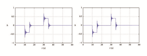
It can be seen from the simulation results in Figure 8 that the water head changes in the pressure pipe are basically the same before and after resampling, which is consistent with actual situation of hydropower plant. Therefore, sampling period contradictions between water diversion pipeline and unit set can be effectively solved by resampling method. Moreover, sampling period of the diversion system can be set arbitrarily and feasibility of real-time simulation of hydroturbine is increased.

4. Study on Convergence of Pressure Loop

A large number of simulation experiments have shown that nonconvergence phenomenon is particularly common in head pressure iteration when the guide vane is fully closed. Therefore, it is necessary to increase convergence of pressure iteration loop to make the results of real-time simulation more accurate and reliable. To solve this problem, sample data of the specific hydroturbine in Section 2.1 are analyzed and processed in this paper firstly; then the BP neural network is used to train and modify these sample data to ensure the smoothness of surface space and continuity of derivative; pressure iteration loop would have better convergence and nonlinear equation can be solved with less iterations by combining with an improved water pressure algorithm proposed in the article. Traditional water pressure algorithm is shown as follows:

()

Relative value of the unit flow can be expressed as follows:

()

Substituting (23) into (19), assume that

()

Then,

()

Define φ as follows:

()

A common method to solve (27) is as follows: start with an estimated value ξ to h_A firstly; then calculate value of φ(ξ) = ξ − D_h(ξ), if φ(ξ) is less than or equal to the standard error set in advance and then iterative end; else ξ = αφ(ξ)+(1 − α)ξ. D_h is defined as follows:

()

To increase algorithm convergence of pressure iteration, an improved method is explored in the paper, and numerical process is as follows.

Equation (24) can be simplified as follows:

()

Substituting (29) into (26),

()

Setting

()

A reasonable solution of (31) should satisfy

. Since A/C ≤ 0 and

are always valid, the only solution is

()

Taking (32) into (26), relative value of pressure can be carried out.

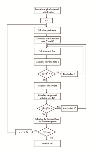
In summary, steps for enhancing pressure loop iteration are as follows: start with an estimated value ξ to h_A in advance; then relative value of flow rate q_A can be obtained by combining with flow and torque neural network training surface; then substitute q_A back into (26) to calculate relative increment value water head pressure Δh_A, if Δh_A is less than or equal to the standard error, iterative end; else, ξ = αφ(ξ)+(1 − α)ξ. Details can be seen in Figure 10.

5. Results and Analysis

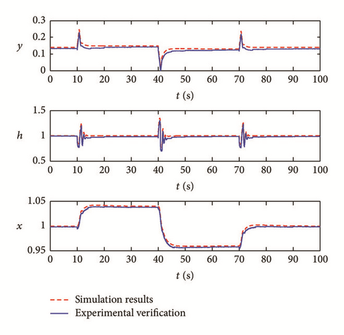
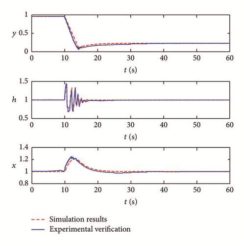
Taking the turbine unit in Section 2.4, for example, hydroturbine governing system suffers 4%, −8%, and 4% frequency disturbance under no-load condition at 10 s, 40 s, and 70 s, respectively. The response of the relay, pressure, frequency is presented in Figure 11(a). It can be seen that elastic water hammer wave can attenuate to a steady state quickly; sampling period and the calculation step of the diversion system can be unified perfectly. Relay, pressure, and frequency response process is shown in Figure 11(b) where the system suffers a 100% load shedding at 10 s. Load rejection and no-load frequency perturbation experiments have been performed at the MHT hydroturbine plant. Model presented above has been used to simulate these transients. Comparisons between measured and computed data are given in Figure 11. The water pressure shows a characteristic of elastic water hammer and has good convergence; head pressure can be controlled to steady state precisely with faster convergence rate. It is worth pointing out that the head pressure has a certain difference with initial value after load shedding because of the energy loss that is caused by a variety of factors, such as friction resistance in the pipeline. Head pressure can recover to original value by modifying the head pressure loss. Simulations and experiments show that synthetic characteristic curve of hydroturbine has been extended successfully and problems existing in real-time simulation are solved effectively by the method proposed in this paper.

6. Summary

Based on analyzing and comparing of advantages and disadvantages of various methods on hydroturbine characteristic curves processing, the BP neural network is applied to the synthetic characteristic curve processing of Francis turbine, and research ideas and methods are introduced in detail. Weights and thresholds of the neural network are obtained with the application examples, and possible causes of errors are analyzed. The obtained weights and thresholds are used as the constant coefficients for polynomial fitting to ensure the nonlinear model be more representative of actual situation. This kind of modeling method can provide not only high precision data for transition process but also better investigation on the real situation of hydraulic unit. Furthermore, this paper performs a detailed analysis and derivation of the improvement of real-time simulation algorithm, including the resampling of the simulation algorithm and iteration convergence of the pressure loop; contradictions of the sampling period between water diversion pipeline and unit set as nonconvergence of the pressure loop are effectively solved finally. Actual engineering applications validate the feasibility of the proposed new method. Further study on the dynamic characteristics of the transition process will be performed in future.

Competing Interests

The authors declare that they have no competing interests.

References

1 Kaldellis J. K., Critical evaluation of the hydropower applications in Greece, Renewable and Sustainable Energy Reviews. (2008) 12, no. 1, 218–234, https://doi.org/10.1016/j.rser.2006.05.003, 2-s2.0-35148891786.
10.1016/j.rser.2006.05.003
Web of Science® Google Scholar
2 Shakya S. R. and Shrestha R. M., Transport sector electrification in a hydropower resource rich developing country: energy security, environmental and climate change co-benefits, Energy for Sustainable Development. (2011) 15, no. 2, 147–159, https://doi.org/10.1016/j.esd.2011.04.003, 2-s2.0-79957513370.
10.1016/j.esd.2011.04.003
CAS Web of Science® Google Scholar
3 Wang B., Xue J., Wu F., and Zhu D., Robust Takagi-Sugeno fuzzy control for fractional order hydro-turbine governing system, ISA Transactions. (2016) 65, 72–80, https://doi.org/10.1016/j.isatra.2016.06.014.
10.1016/j.isatra.2016.06.014
PubMed Web of Science® Google Scholar
4 Zeng Y., Zhang L., Guo Y., Qian J., and Zhang C., The generalized Hamiltonian model for the shafting transient analysis of the hydro turbine generating sets, Nonlinear Dynamics. (2014) 76, no. 4, 1921–1933, https://doi.org/10.1007/s11071-014-1257-9, ZBL1314.37057, 2-s2.0-84902535684.
10.1007/s11071?014?1257?9
Web of Science® Google Scholar
5 Ren M., Wu D., Zhang J., and Jiang M., Minimum entropy-based cascade control for governing hydroelectric turbines, Entropy. (2014) 16, no. 6, 3136–3148, https://doi.org/10.3390/e16063136.
10.3390/e16063136
Web of Science® Google Scholar
6 Khodabakhshian A. and Hooshmand R., A new PID controller design for automatic generation control of hydro power systems, International Journal of Electrical Power and Energy Systems. (2010) 32, no. 5, 375–382, https://doi.org/10.1016/j.ijepes.2009.11.006, 2-s2.0-77949567089.
10.1016/j.ijepes.2009.11.006
Web of Science® Google Scholar
7 Li C., Chang L., Huang Z., Liu Y., and Zhang N., Parameter identification of a nonlinear model of hydraulic turbine governing system with an elastic water hammer based on a modified gravitational search algorithm, Engineering Applications of Artificial Intelligence. (2016) 50, 177–191, https://doi.org/10.1016/j.engappai.2015.12.016, 2-s2.0-84960122727.
10.1016/j.engappai.2015.12.016
Web of Science® Google Scholar
8 Wang X., Lin S., and Wang S., Dynamic friction parameter identification method with lugre model for direct-drive rotary torque motor, Mathematical Problems in Engineering. (2016) 2016, 8, 6929457, https://doi.org/10.1155/2016/6929457, 2-s2.0-84964727144.
10.1155/2016/6929457
Web of Science® Google Scholar
9 Zhang N., Li C., Li R., Lai X., and Zhang Y., A mixed-strategy based gravitational search algorithm for parameter identification of hydraulic turbine governing system, Knowledge-Based Systems. (2016) 109, 218–237, https://doi.org/10.1016/j.knosys.2016.07.005, 2-s2.0-84978900458.
10.1016/j.knosys.2016.07.005
Web of Science® Google Scholar
10 Chen D., Ding C., Ma X., Yuan P., and Ba D., Nonlinear dynamical analysis of hydro-turbine governing system with a surge tank, Applied Mathematical Modelling. (2013) 37, no. 14-15, 7611–7623, https://doi.org/10.1016/j.apm.2013.01.047, MR3089581, 2-s2.0-84880646277.
10.1016/j.apm.2013.01.047
Web of Science® Google Scholar
11 Guo W., Yang J., Chen J., and Wang M., Nonlinear modeling and dynamic control of hydro-turbine governing system with upstream surge tank and sloping ceiling tailrace tunnel, Nonlinear Dynamics. (2016) 84, no. 3, 1383–1397, https://doi.org/10.1007/s11071-015-2577-0, MR3486576, 2-s2.0-84953392410.
10.1007/s11071?015?2577?0
Web of Science® Google Scholar
12 Xiao Z., He X., Fu X., and Malik O. P., ACO-initialized wavelet neural network for vibration fault diagnosis of hydroturbine generating unit, Mathematical Problems in Engineering. (2015) 2015, 7, 354658, https://doi.org/10.1155/2015/354658, 2-s2.0-84942811426.
10.1155/2015/354658
Web of Science® Google Scholar
13 Zhang P., Chen G., and Zhang X., Application of BP neural network and RBF neural network in extending hydraulic turbine combined characteristic curve, China Rural Water and Hydropower. (2012) 11, no. 35, 125–131.
Google Scholar
14 Pennacchi P., Chatterton S., and Vania A., Modeling of the dynamic response of a Francis turbine, Mechanical Systems and Signal Processing. (2012) 29, 107–119, https://doi.org/10.1016/j.ymssp.2011.05.012, 2-s2.0-84859419324.
10.1016/j.ymssp.2011.05.012
Web of Science® Google Scholar
15 Huang X. and Liu D., The treatment of hydroturbine synthetic characteristic curve by radial basis networks, Journal of Hydroelectric Engineering. (2007) 26, no. 1, 114–118, 2-s2.0-33947537449.
Google Scholar
16 Yuanchu C., Luqing Y., and Weiyou C., Modeling of hydro-turbine hill chart by neural network, Journal of Huazhong University of Science and Technology (Nature Science Edition). (2003) 31, no. 6, 68–70.
Google Scholar
17 Zhang R., Liu Z., Wang L., and Zhang Y., Data interpolation by Delaunay triangulation for the combined characteristic curve of a turbine, Journal of Hydroelectric Engineering. (2011) 30, no. 4, 197–221, 2-s2.0-82055204916.
Google Scholar

Citing Literature

All articles

A New Processing Method Combined with BP Neural Network for Francis Turbine Synthetic Characteristic Curve Research

Abstract

1. Introduction

2. Synthetic Characteristic Curve Processing Method of Francis Turbine