Volume 2016, Issue 1 6390367
Research Article
Open Access

A New Accurate and Efficient Iterative Numerical Method for Solving the Scalar and Vector Nonlinear Equations: Approach Based on Geometric Considerations

Grégory Antoni

Corresponding Author

Grégory Antoni

Aix-Marseille Université, IFSTTAR, LBA UMR T24, 13016 Marseille, France univ-amu.fr

Search for more papers by this author
First published: 07 August 2016
Citations: 2
Academic Editor: Josè A. Tenereiro Machado

Abstract

This paper deals with a new numerical iterative method for finding the approximate solutions associated with both scalar and vector nonlinear equations. The iterative method proposed here is an extended version of the numerical procedure originally developed in previous works. The present study proposes to show that this new root-finding algorithm combined with a stationary-type iterative method (e.g., Gauss-Seidel or Jacobi) is able to provide a longer accurate solution than classical Newton-Raphson method. A numerical analysis of the developed iterative method is addressed and discussed on some specific equations and systems.

1. Introduction

Solving both nonlinear equations and systems is a situation very often encountered in various fields of formal or physical sciences. For instance, solid mechanics is a branch of physics where the resolution of problems governed by nonlinear equations and systems occurs frequently [110]. In most cases, Newton method (also known as Newton-Raphson algorithm) is most commonly used for approximating the solutions of scalar and vector nonlinear equations [1113]. But, over the years, several other numerical methods have been developed for providing iteratively the approximate solutions associated with nonlinear equations and/or systems [1425]. Some of them present the advantage of having both high accuracy and strong efficiency using a numerical procedure based on an enhanced Newton-Raphson algorithm [26]. In this study, we propose to improve the iterative procedure developed in previous works [27, 28] for finding numerically the solution of both scalar and vector nonlinear equations. This study is decomposed as follows: (i) in Section 2, a new numerical geometry-based root-finding algorithm coupled with a stationary-type iterative method (such as Jacobi or Gauss-Seidel) is presented with the aim of solving any system of nonlinear equations [29, 30]; (ii) in Section 3, the numerical predictive abilities associated with the proposed iterative method are tested on some examples and also compared with other algorithms [31, 32].

2. New Iterative Numerical Method for Solving the Scalar and Vector Nonlinear Equations Based on a Geometric Approach

2.1. Problem Statement

We consider vector-valued function , which is continuous and infinitely differentiable (i.e., ), checking the following equation:
()
where X = trans({x1, x2, x3, …, xn}) denotes the vector-valued variable (with ), xi is ith component associated with vector X (with 1 ≤ in), trans(⋆) is the transpose operator associated with the variable ⋆, and denotes the class of infinitely differentiable functions in domain Ω. It should be mentioned that: (i) the nonlinear function has a unique solution X on domain Ω which is an open subset of , that is, such as ; (ii) the case of scalar equation (f) with only one variable (x) is obtained when n = 1, that is, .
Equation (1) can also rewritten as system of n-scalar nonlinear equations, that is,
()
where Fi denotes ith component associated with vector-valued function F (see (1)), that is, ith nonlinear equation of system . It should be noted that: (i) in the case of i ∈ [1, n] (with n > 1), the nonlinear system (2) has a unique solution set such as ; (ii) in the case of n = 1, nonlinear system (2) is transformed in scalar nonlinear equation which has a unique solution x such as f(x) = 0; (iii) (1) and (2) are mathematically equivalent, that is, .

With the aim of numerically solving system (2), we adopt a Root-Finding Algorithm (RFA) coupled with a Stationary Iterative Procedure (SIP) such as Jacobi or Gauss-Seidel [26, 30]. The use of any SIP allows to reduce the considered nonlinear system to a successive set of nonlinear equations with only one variable and therefore it can be solved with a RFA [30]. In the present study, we propose an extended version of RFA already developed in [27, 28] and combined with a Jacobi or Gauss-Seidel type iterative procedure for dealing any system of nonlinear equations.

2.2. Stationary Iterative Procedures (SIPs) with Root-Finding Algorithms (RFAs)

2.2.1. Jacobi and Gauss-Seidel Iterative Procedures

In order to solve a system of nonlinear equations, any RFA can be used if it is combined with a SIP (i.e., Jacobi or Gauss-Seidel) [26, 29, 30]. A Jacobi or Gauss-Seidel type procedure applied to nonlinear system (1) can be described as follows:
()
with
  • (i)

    in the case of Jacobi procedure:

    ()

  • (ii)

    in the case of Gauss-Seidel procedure:

    ()

where ⋆k (resp., ⋆k+1) denotes kth (resp., (k + 1)th) iteration associated with the variable ⋆ (), Δi is the set of kept constant variables, and {†} represents one set of variables †.

2.3. Used Root-Finding Algorithm (RFA)

In previous works [27, 28], a root-finding algorithm (RFA) has been developed for approximating the solutions of scalar nonlinear equations. The new RFA presented here is an extended version to that previously developed taking into account some geometric considerations. In this paper, we propose to use a RFA coupled with Jacobi and Gauss-Seidel type procedures for iteratively solving nonlinear system . Hence, we adopt a new RFA for finding approximate solution (when i is fixed and with the known set Δi) associated with each nonlinear equation Fi of system (see Section 2.1). For each nonlinear equation Fi, parametrized by the set of variables Δi, depending only on one variable , we introduce the exact and inexact local curvature associated with the curve representing the nonlinear equation in question.

The used RFA is based on the following main steps (see [27] for more details):
  • (i)

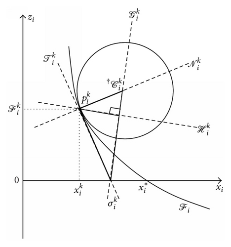
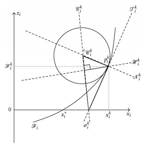
    In the first step, we consider the iterative tangent and normal straight lines associated with nonlinear function Fi at point (see Figure 1):

    ()

  • where (resp., ) denotes the value (resp., first-order derivative) of function Fi at point , is the set of known variables and (Ti, Ni) are two functionals associated with .

  • (ii)

    In the second step, we introduce the iterative exact and inexact local curvature associated with the curve representing nonlinear function at point (see Figure 1):

    ()

  • where |∗| denotes the absolute-value function associated with the variable ∗, is the exact († = ex) or inexact († = in) radius of the osculating at point , (with † = ex, in) is functional associated with , and is the second-order derivative of function Fi at point . It should be noted that: (i) we consider the exact radius associated with the true osculating circle at point (see [33]); (ii) in line with [27, 28], we consider an inexact radius associated with the osculating circle at point , that is, (see (7)).

  • (iii)

    In the third step, we define the iterative center associated with the exact and inexact osculating circle at point , that is, (see Figure 1)

    ()

  • By taking (7) and (8), the iterative centers are (with † = ex, in)

    ()

  • where is the iterative centers associated with the exact and inexact osculating circle (with † = ex, in) associated with each curve representing nonlinear function at point , are two functionals associated with and sgn⁡() is sign function (i.e., sgn⁡() = −1 when < 0, sgn() = 1 when > 0, and sgn() = 0 when = 0).

  • (iv)

    In the fourth step, we introduce the iterative point such as , that is,

    ()

  • where Wi is a functional associated with .

  • (v)

    In the fifth step, we define the iterative straight line passing through two iterative points and , that is, (with † = ex, in)

    ()

  • where is the set of known variables.

  • (vi)

    In the sixth step, we introduce the iterative straight line passing through the point and the iterative perpendicular straight line such as (with † = ex, in)

    ()

  • where Hi is a functional associated with .

  • (vii)

    In the last step, we define the iterative point which is the solution of the following relation (with † = ex, in)

    ()

  • with

    ()

  • where Pi is a functional associated with Φi.

  • In line with (10), (14) can be rewritten as

    ()
Details are in the caption following the image
Schematic diagram with the specific entities used by the new RFA applied on ith component Fi associated with system in the case of monotonically increasing (a) and decreasing (b) evolution with the known set of parameters Δi.
Details are in the caption following the image
Schematic diagram with the specific entities used by the new RFA applied on ith component Fi associated with system in the case of monotonically increasing (a) and decreasing (b) evolution with the known set of parameters Δi.
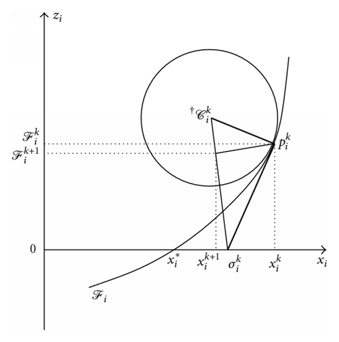
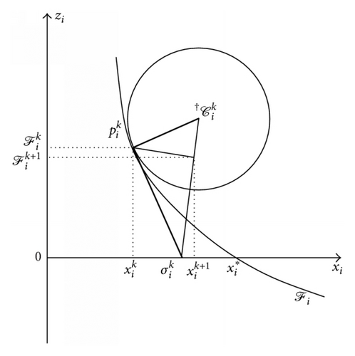
The new iterative method that we will thereafter appoint as “Adaptative Geometric-based Algorithm” (AGA) enables providing a more convenient approximate solution associated with a system of nonlinear equations of type , that is, (see Figure 2)
()
with
()
and for conditions [BC1], [BC2], [BC4], and [BC5]:
()
and for conditions [BC3] and [BC6]:
()
where Γ denotes the fixed-point function [13] used to the considered RFA (i.e., AGA) and is the set of known variables.
Details are in the caption following the image
Geometric interpretation of the new RFA (i.e., AGA) applied on ith component Fi associated with system in the case of monotonically increasing (a) and decreasing (b) evolution with the known set of parameters Δi.
Details are in the caption following the image
Geometric interpretation of the new RFA (i.e., AGA) applied on ith component Fi associated with system in the case of monotonically increasing (a) and decreasing (b) evolution with the known set of parameters Δi.
The different conditions [BC] associated with the proposed RFA (i.e., AGA) are as follows:
  • (i)

    First condition [BC1] is

    ()

  • (ii)

    Second condition [BC2] is

    ()

  • (iii)

    Third condition [BC3] is

    ()

  • (iv)

    Fourth condition [BC4] is

    ()

  • (v)

    Fifth condition [BC5] is

    ()

  • (vi)

    Sixth condition [BC6] is

    ()

3. Numerical Examples

3.1. Preliminary Remarks

In this section, we propose to evaluate the predictive abilities associated with the numerical iterative method developed in Section 2.3 (i.e., AGA) on some examples both in the case of scalar and vector nonlinear equations. Hence, AGA is compared to other iterative Newton-Raphson type methods [27, 28, 3032] coupled with Jacobi (J) and Gauss-Seidel (GS) techniques. All the numerical implementations associated with these presented iterative methods have been made in Matlab software (see [26, 3439]).

The used iterative methods for the different examples are as follows (see [27, 28, 3032]):
  • (i)

    Newton-Raphson Algorithm (NRA):

    ()

  • where denotes the first-order differential operator associated with nonlinear function F at point and inv(†) is the inverse transform operator of †. It is important to highlight that NRA can be used if and only if operator “” exists, that is, , (det⁡(‡) is determinant of operator ‡).

  • (ii)

    Standard Newton’s Algorithm (SNA):

    ()

  • (iii)

    Third-order Modified Newton Method (TMNM):

    ()

In order to stop the iterative process associated with each considered algorithm, we consider three coupled types of criteria for dealing with nonlinear equations:
  • (i)

    For scalar-valued equations :

    • (a)

      (C1S) on the iteration number,

      ()

    • where denotes the maximum number of iterations associated with scalar-valued equations.

    • (b)

      (C2S) on the residue error,

      ()

    • where is the tolerance parameter associated with the residue error criterion for scalar-valued equations and ‖†‖ = |†| is the absolute-value norm.

    • (c)

      (C3S) on the approximation error,

      ()

    • where is the tolerance parameter associated with the absolute error criterion for scalar-valued equations.

  • (ii)

    For vector-valued equations :

    • (a)

      (C1V) on the iteration number, we adopt the same condition that (C1S), that is, (where denotes the maximum number of iterations associated with vector-valued equations).

    • (b)

      (C2V) on the residue error,

      ()

    • where (resp., ) is the tolerance parameter associated with the residue error criterion for vector-valued equations and is the vector p-norm (here, p = 1,2). It is important to point out that is so-called Euclidean norm.

    • (c)

      (C3V) on the approximation error,

      ()

    • where ϵae is the tolerance parameter associated with the absolute error criterion for vector-valued equations.

Here, for the stopping criteria (C1S, C1V), (C2S, C2V), and (C3S, C3V) associated with the iterative process, we consider: (i) the maximum number of iterations ; (ii) the tolerance parameter for the scalar-valued equations; (iii) the tolerance parameter (with i = 1,2) for the vector-valued equations.

3.2. Examples

We consider the following nonlinear equations.
  • (i)

    In case n = 1 (i.e., scalar-valued equations), one has the following:

Example 1. Consider the following:

()

Example 2. Consider the following:

()
  • (ii)

    In case n = 2 (i.e., vector-valued equations), one has the following:

Example 3. Consider the following:

()

Example 4. Consider the following:

()

3.3. Results and Discussion

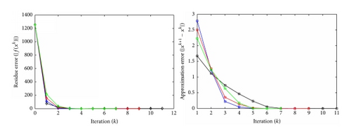
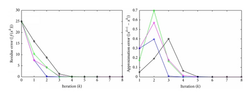
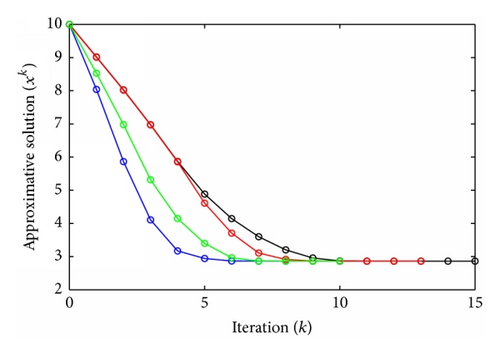
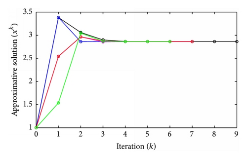
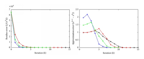
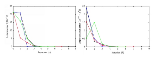
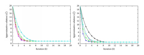
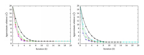
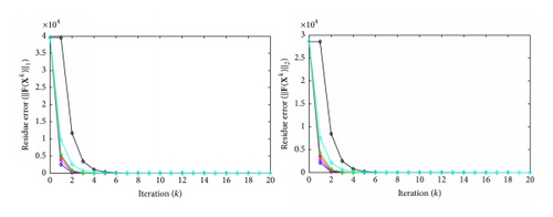
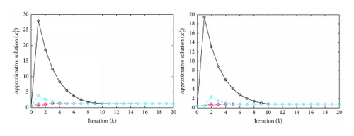
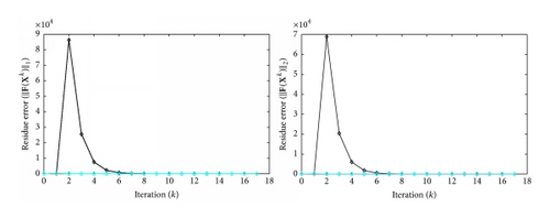
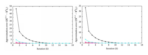
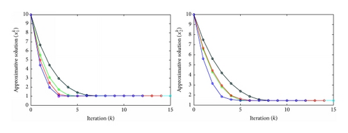
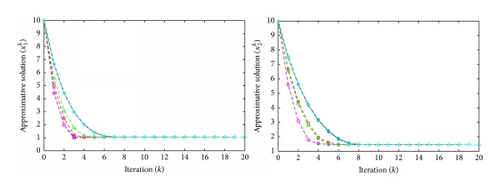
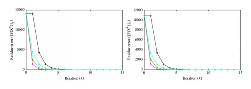
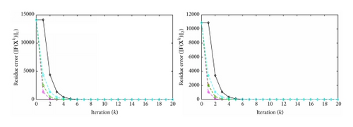
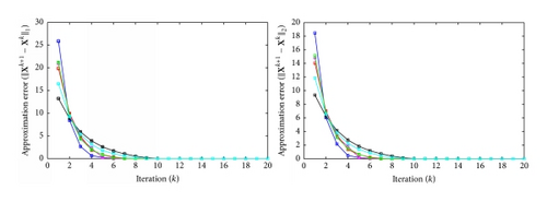
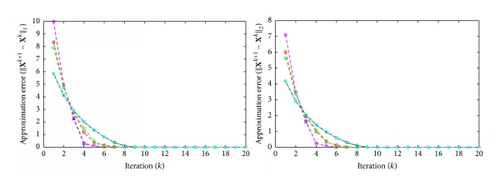
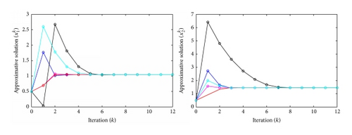
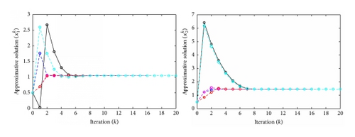
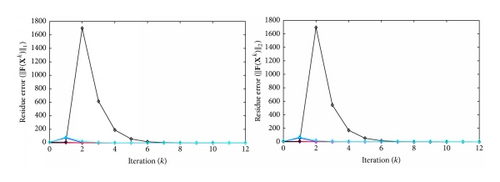
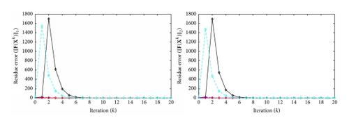
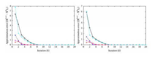
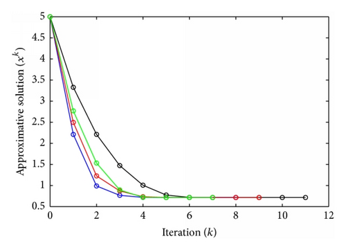
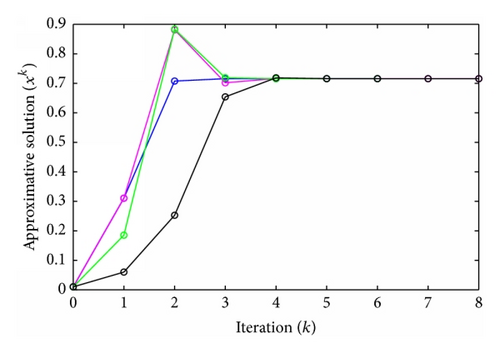
All the numerical results of Examples 14 are shown in Figures 332. For Example 1 (resp., Example 2) with guest start point (resp., ), we can see that approximate solutions provided by AGA with condition [BC1]/[BC3] (i.e., condition [BC1] is the same that [BC3] where † = ex) are better than AGA with condition [BC2], NRA/SNA (when n = 1, NRA and SNA are the same), and TMNM. For Example 1 (resp., Example 2) in the case of guest start point (resp., ), we can see that approximate solutions provided by AGA with conditions [BC4], [BC5], and [BC6] in the first iterations are accurately better than NRA/SNA (when n = 1, NRA and SNA are the same) and TMNM. For Example 3 with guest start point couple , we can observe that approximate solutions given by AGA using Gauss-Seidel (GS) or Jacobi (J) procedure with: (i) condition [BC1] are more accurate numerically than NRA, TMNM, and SNA; (ii) conditions [BC2] and [BC3] are accurately better than NRA (only in the first iterations) and SNA. In the case of guest start point couple , we can see that approximate solutions provided by AGA using: (i) Gauss-Seidel (GS) procedure with condition [BC6] give much greater numerical accuracy than NRA and SNA; (ii) Gauss-Seidel (GS) procedure with conditions [BC4] and [BC5] offer much greater numerical accuracy than NRA and SNA; (iii) Jacobi (J) procedure with conditions [BC4], [BC5], and [BC6] are better than NRA (only in the first iterations) and SNA. For Example 4 with guest start point couple , we can see that approximate solutions given by AGA using: (i) Gauss-Seidel (GS) procedure with conditions [BC1] and [BC3] are more accurate numerically than SNA, TMNM, and NRA; (ii) Gauss-Seidel (GS) procedure with condition [BC2] are accurately better than TMNM and NRA (only in the first iterations) and SNA; (iii) Jacobi (J) procedure with conditions [BC1], [BC2], and [BC3] are more accurate numerically than NRA (only in the first iterations) and both TMNM and SNA. In the case of guest start point couple , approximate solutions obtained by AGA using: (i) Gauss-Seidel (GS) procedure with conditions [BC5] and [BC6] are more accurate numerically than SNA and NRA; (ii) Jacobi (J) procedure with the conditions [BC4], [BC5], and [BC6] are accurately better than NRA (only in the first iterations) and SNA. Overview of different numerical results shows that the Adaptive Geometry-based Algorithm (AGA) can be able to provide quite accurately the approximate solutions associated with both nonlinear equations and systems and can potentially provide a better or more suitable approximate solution than that of Newton-Raphson Algorithm (NRA).
Details are in the caption following the image
Evolution of approximate solutions xk associated with () compared to kth iteration for Example 1 (where x0 = 5) with NRA/SNA (black solid line with circles), TMNM (green solid line with circles), and AGA with condition [BC1]/[BC3] (blue solid line with circles) and condition [BC2] (red solid line with circles).
Details are in the caption following the image
Evolution of approximate solutions xk associated with () compared to kth iteration for Example 1 (where x0 = 10−2) with NRA/SNA (black solid line with circles), TMNM (green solid line with circles), and AGA with condition [BC4] (blue solid line with circles) and condition [BC5]/[BC6] (magenta solid line with circles).
Details are in the caption following the image
Evolution of residue error (C2S) and approximation error (C3S) associated with () compared to kth iteration for Example 1 (where x0 = 5) with NRA/SNA (black solid line with diamonds and squares), TMNM (green solid line with diamonds and squares), and AGA with condition [BC1]/[BC3] (blue solid line with diamonds and squares) and condition [BC2] (red solid line with diamonds and squares).
Details are in the caption following the image
Evolution of residue error (C2S) and approximation error (C3S) associated with () compared to kth iteration for Example 1 (where x0 = 10−2) with NRA/SNA (black solid line with diamonds and squares), TMNM (green solid line with diamonds and squares), and AGA with condition [BC4] (blue solid line with diamonds and squares) and condition [BC5]/[BC6] (magenta solid line with diamonds and squares).
Details are in the caption following the image
Evolution of approximate solutions xk associated with () compared to kth iteration for Example 2 (where x0 = 10) with NRA/SNA (black solid line with circles), TMNM (green solid line with circles), and AGA with condition [BC1]/[BC3] (blue solid line with circles) and condition [BC2] (red solid line with circles).
Details are in the caption following the image
Evolution of approximate solutions xk associated with () compared to kth iteration for Example 2 (where x0 = 1) with NRA/SNA (black solid line with circles), TMNM (green solid line with circles), and AGA with condition [BC4] (blue solid line with circles), condition [BC5] (red solid line with circles), and condition [BC6] (magenta solid line with circles).
Details are in the caption following the image
Evolution of residue error (C2S) and approximation error (C2S) associated with () compared to kth iteration for Example 1 (where x0 = 10) with NRA/SNA (black solid line with diamonds and squares), TMNM (green solid line with diamonds and squares), and AGA with condition [BC1]/[BC3] (blue solid line with diamonds and squares) and condition [BC2] (red solid line with diamonds and squares).
Details are in the caption following the image
Evolution of residue error (C2S) and approximation error (C3S) associated with () compared to kth iteration for Example 2 (where x0 = 1) with NRA/SNA (black solid line with diamonds and squares), TMNM (green solid line with diamonds and squares), and AGA with condition [BC4] (blue solid line with diamonds and squares), condition [BC5] (red solid line with diamonds and squares), and condition [BC6] (magenta solid line with diamonds and squares).
Details are in the caption following the image
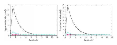
Evolution of approximate solutions () associated with () compared to kth iteration for Example 3 (where ) with NRA (black solid line with circles) and some other algorithms coupled with Gauss-Seidel (GS) procedure: SNA-GS (cyan solid line with circles), TMNM-GS (green solid line with circles), AGA-GS with condition [BC1] (blue solid line with circles), condition [BC2] (red solid line with circles), and condition [BC3] (magenta solid line with circles).
Details are in the caption following the image
Evolution of approximate solutions () associated with () compared to kth iteration for Example 3 (where ) with NRA (black solid line with circles) and some other algorithms coupled with Jacobi (J) procedure: SNA-J (cyan dashed line with circles), TMNM-J (green dashed line with circles), and AGA-J with condition [BC1] (blue dashed line with circles), condition [BC2] (red dashed line with circles), and condition [BC3] (magenta dashed line with circles).
Details are in the caption following the image
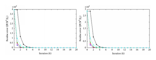
Evolution of residue error using (C2V1) and (C2V2) conditions associated with () compared to kth iteration for Example 3 (where ) with NRA (black solid line with diamonds) and some other algorithms coupled with Gauss-Seidel (GS) procedure: SNA-GS (cyan solid line with diamonds), TMNM-GS (green solid line with diamonds), and AGA-GS with condition [BC1] (blue solid line with diamonds), condition [BC2] (red solid line with diamonds), and condition [BC3] (magenta solid line with diamonds).
Details are in the caption following the image
Evolution of residue error using (C2V1) and (C2V2) conditions associated with () compared to kth iteration for Example 3 (where ) with NRA (black solid line with diamonds) and some other algorithms coupled with Jacobi (J) procedure: SNA-J (cyan dashed line with diamonds), TMNM-J (green dashed line with diamonds), and AGA-J with condition [BC1] (blue dashed line with diamonds), condition [BC2] (red dashed line with diamonds), and condition [BC3] (magenta dashed line with diamonds).
Details are in the caption following the image
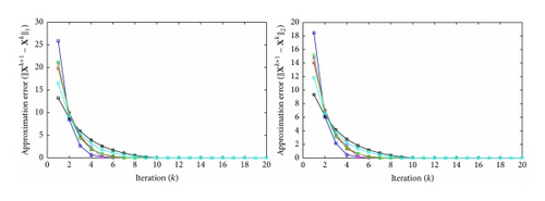
Evolution of the approximation error using (C3V1) and (C3V2) conditions associated with () compared to kth iteration for Example 3 (where ) with NRA (black solid line with squares) and some other algorithms coupled with Gauss-Seidel (GS) procedure: SNA-GS (cyan solid line with squares), TMNM-GS (green solid line with squares), and AGA-GS with condition [BC1] (blue solid line with squares), condition [BC2] (red solid line with squares), and condition [BC3] (magenta solid line with squares).
Details are in the caption following the image
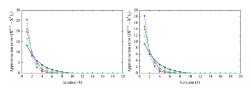
Evolution of the approximation error using (C3V1) and (C3V2) conditions associated with () compared to kth iteration for Example 3 (where ) with NRA (black solid line with squares) and some other algorithms coupled with Jacobi (J) procedure: SNA-J (cyan dashed line with squares), TMNM-J (green dashed line with squares), and AGA-J with condition [BC1] (blue dashed line with squares), condition [BC2] (red dashed line with squares), and condition [BC3] (magenta dashed line with squares).
Details are in the caption following the image
Evolution of approximate solutions () associated with () compared to kth iteration for Example 3 (where ) with NRA (black solid line with circles) and some other algorithms coupled with Gauss-Seidel (GS) procedure: SNA-GS (cyan solid line with circles) and AGA-GS with condition [BC4] (blue solid line with circles), condition [BC5] (red solid line with circles), and condition [BC6] (magenta solid line with circles).
Details are in the caption following the image
Evolution of approximate solutions () associated with () compared to kth iteration for Example 3 (where ) with NRA (black solid line with diamonds and squares) and some other algorithms coupled with Jacobi (J) procedure: SNA-J (cyan dashed line with circles) and AGA-J with condition [BC4] (blue dashed line with circles), condition [BC5] (red dashed line with circles), and condition [BC6] (magenta dashed line with circles).
Details are in the caption following the image
Evolution of residue error using (C2V1) and (C2V2) conditions associated with () compared to kth iteration for Example 3 (where ) with NRA (black line) and some other algorithms coupled with Gauss-Seidel (GS) and Jacobi (J) procedures: SNA-GS/SNA-J (cyan line) and AGA-GS/AGA-J with condition [BC4] (blue line), condition [BC5] (red line), and condition [BC6] (magenta line).
Details are in the caption following the image
Evolution of approximation error for (C3V1) and (C3V2) conditions associated with () compared to kth iteration for Example 3 (where ) with NRA (black line) and some other algorithms coupled with Gauss-Seidel (GS) and Jacobi (J) procedures: SNA-GS/SNA-J (cyan line) and AGA-GS/AGA-J with condition [BC4] (blue line), condition [BC5] (red line), and condition [BC6] (magenta line).
Details are in the caption following the image
Evolution of approximate solutions () associated with () compared to kth iteration for Example 4 (where ) with NRA (black solid line with circles) and some other algorithms coupled with Gauss-Seidel (GS) procedure: SNA-GS (cyan solid line with circles), TMNM-GS (green solid line with circles), and AGA-GS with condition [BC1] (blue solid line with circles), condition [BC2] (red solid line with circles), and condition [BC3] (magenta solid line with circles).
Details are in the caption following the image
Evolution of approximate solutions () associated with () compared to kth iteration for Example 4 (where ) with NRA (black solid line with circles) and some other algorithms coupled with Jacobi (J) procedure: SNA-J (cyan dashed line with circles), TMNM-J (green dashed line with circles), and AGA-J with condition [BC1] (blue dashed line with circles), condition [BC2] (red dashed line with circles), and condition [BC3] (magenta dashed line with circles).
Details are in the caption following the image
Evolution of residue error using (C2V1) and (C2V2) conditions associated with () compared to kth iteration for Example 4 (where ) with NRA (black solid line with diamonds) and some other algorithms coupled with Gauss-Seidel (GS) procedure: SNA-GS (cyan solid line with diamonds), TMNM-GS (green solid line with diamonds), and AGA-GS with condition [BC1] (blue solid line with diamonds), condition [BC2] (red solid line with diamonds), and condition [BC3] (magenta solid line with diamonds).
Details are in the caption following the image
Evolution of residue error using (C2V1) and (C2V2) conditions associated with () compared to kth iteration for Example 4 (where ) with NRA (black solid line with diamonds) and some other algorithms coupled with Jacobi (J) procedure: SNA-J (cyan dashed line with diamonds), TMNM-J (green dashed line with diamonds), and AGA-J with condition [BC1] (blue dashed line with diamonds), condition [BC2] (red dashed line with diamonds), and condition [BC3] (magenta dashed line with diamonds).
Details are in the caption following the image
Evolution of the approximation error using (C3V1) and (C3V2) associated with () compared to kth iteration for Example 4 (where ) with NRA (black solid line with squares) and some other algorithms coupled with Gauss-Seidel (GS) procedure: SNA-GS (cyan solid line with squares), TMNM-GS (green solid line with squares), and AGA-GS with condition [BC1] (blue solid line with squares), condition [BC2] (red solid line with squares), and condition [BC3] (magenta solid line squares).
Details are in the caption following the image
Evolution of the approximation error using (C3V1) and (C3V2) conditions associated with () compared to kth iteration for Example 4 (where ) with NRA (black solid line with squares) and some other algorithms coupled with Jacobi (J) procedure: SNA-J (cyan dashed line with squares), TMNM-J (green dashed line with squares), and AGA-J with condition [BC1] (blue dashed line with squares), condition [BC2] (red dashed line with squares), and condition [BC3] (magenta dashed line with squares).
Details are in the caption following the image
Evolution of approximate solutions () associated with () compared to kth iteration for Example 4 (where ) with NRA (black solid line with circles) and some other algorithms coupled with Gauss-Seidel (GS) procedure: SNA-GS (cyan solid line with circles) and AGA-GS with condition [BC4] (blue solid line with circles), condition [BC5] (red solid line with circles), and condition [BC6] (magenta solid line with circles).
Details are in the caption following the image
Evolution of approximate solutions () associated with () compared to kth iteration for Example 4 (where ) with NRA (black solid line with circles) and some other algorithms coupled with Jacobi (J) procedure: SNA-J (cyan dashed line with circles) and AGA-J with condition [BC4] (blue dashed line with circles), condition [BC5] (red dashed line with circles), and condition [BC6] (magenta dashed line with circles).
Details are in the caption following the image
Evolution of the residue error using (C2V1) and (C2V2) conditions associated with () compared to kth iteration for Example 4 (where ) with NRA (black solid line with diamonds) and some other algorithms coupled with Gauss-Seidel (GS) procedure: SNA-GS (cyan solid line with diamonds) and AGA-GS with condition [BC4] (blue solid line with diamonds), condition [BC5] (red solid line with diamonds), and condition [BC6] (magenta solid line with diamonds).
Details are in the caption following the image
Evolution of residue error using (C2V1) and (C2V2) conditions associated with () compared to kth iteration for Example 4 (where ) with NRA (black solid line with diamonds) and some other algorithms coupled with Jacobi (J) procedure: SNA-J (cyan dashed line with diamonds) and AGA-J with condition [BC4] (blue dashed line with diamonds), condition [BC5] (red dashed line with diamonds), and condition [BC6] (magenta dashed line with diamonds).
Details are in the caption following the image
Evolution of approximation error using (C3V1) and (C3V2) conditions associated with () compared to kth iteration for Example 4 (where ) with NRA (black solid line with squares) and some other algorithms coupled with Gauss-Seidel (GS) procedure: SNA-GS (cyan solid line with squares) and AGA-GS with condition [BC4] (blue solid line with squares), condition [BC5] (red solid line with squares), and condition [BC6] (magenta solid line with squares).
Details are in the caption following the image
Evolution of the approximation error using (C3V1) and (C3V2) conditions associated with () compared to kth iteration for Example 4 (where ) with NRA (black solid line with squares) and some other algorithms coupled with Jacobi (J) procedure: SNA-J (cyan dashed line with squares) and AGA-J with condition [BC4] (blue dashed line with squares), condition [BC5] (red dashed line with squares), and condition [BC6] (magenta dashed line with squares).

4. Concluding Comments

The present work concerns a new numerical iterative method for approximating the solutions of both scalar and vector nonlinear equations. Based on an iterative procedure previously developed in a study, we propose here an extended form of this numerical algorithm including the use of a stationary-type iterative procedure in order to solve systems of nonlinear equations. A predictive numerical analysis associated with this proposed method for providing a more accurate approximate solution in regard to nonlinear equations and systems is tested, assessed and discussed on some specific examples.

Competing Interests

The author declares that there are no competing interests regarding the publication of this paper.

    The full text of this article hosted at iucr.org is unavailable due to technical difficulties.