International Journal of Differential Equations

Volume 2016, Issue 1 2010464

Research Article

Open Access

The Dynamical Analysis of a Prey-Predator Model with a Refuge-Stage Structure Prey Population

Raid Kamel Naji,

Raid Kamel Naji

Department of Mathematics, College of Science, Baghdad University, Baghdad, Iraq uobaghdad.edu.iq

Search for more papers by this author

Salam Jasim Majeed,

Corresponding Author

Salam Jasim Majeed

[email protected]

orcid.org/0000-0001-9550-150X

Department of Mathematics, College of Science, Baghdad University, Baghdad, Iraq uobaghdad.edu.iq

Department of Physics, College of Science, Thi-Qar University, Nasiriyah, Iraq utq.edu.iq

Search for more papers by this author

Raid Kamel Naji,

Raid Kamel Naji

Department of Mathematics, College of Science, Baghdad University, Baghdad, Iraq uobaghdad.edu.iq

Search for more papers by this author

Salam Jasim Majeed,

Corresponding Author

Salam Jasim Majeed

[email protected]

orcid.org/0000-0001-9550-150X

Department of Mathematics, College of Science, Baghdad University, Baghdad, Iraq uobaghdad.edu.iq

Department of Physics, College of Science, Thi-Qar University, Nasiriyah, Iraq utq.edu.iq

Search for more papers by this author

First published: 24 November 2016

https://doi.org/10.1155/2016/2010464

Citations: 17

Academic Editor: Jaume Giné

Share a link

Email
Wechat
Bluesky

Abstract

We proposed and analyzed a mathematical model dealing with two species of prey-predator system. It is assumed that the prey is a stage structure population consisting of two compartments known as immature prey and mature prey. It has a refuge capability as a defensive property against the predation. The existence, uniqueness, and boundedness of the solution of the proposed model are discussed. All the feasible equilibrium points are determined. The local and global stability analysis of them are investigated. The occurrence of local bifurcation (such as saddle node, transcritical, and pitchfork) near each of the equilibrium points is studied. Finally, numerical simulations are given to support the analytic results.

1. Introduction

The development of the qualitative analysis of ordinary differential equations is deriving to study many problems in mathematical biology. The modeling for the population dynamics of a prey-predator system is one of the important and interesting goals in mathematical biology, which has received wide attention by several authors [1–6]. In the natural world many kinds of prey and predator species have a life history that is composed of at least two stages: immature and mature, and each stage has different behavioral properties. So, some works of stage structure prey-predator models have been provided in a good number of papers in the literatures [7–12]. Zhang et al. in [9] and Cui and Takeuchi in [11] proposed two mathematical models of prey stage structure; in these models the predator species consumes exclusively the immature prey. Indeed, there are many factors that impact the dynamics of prey-predator interactions such as disease, harvesting, prey refuge, delay, and many other factors. Several prey species have gone to extinction, and this extinction must be caused by external effects such as overutilization, overpredation, and environmental factors (pollution, famine). Prey may avoid becoming attacked by predators either by protecting themselves or by living in a refuge where it will be out of sight of predators. Some theoretical and empirical studies have shown and tested the effects of prey refuges and making an opinion that the refuges used by prey have a stabilizing influence on prey-predator interactions; also prey extinction can be prevented by the addition of refuges; for instance, we can refer to [13–23]. Therefore, it is important and worthwhile to study the effects of a refuge on the prey population with prey stage structure. Consequently, in this paper, we proposed and analyzed the prey-predator model involving a stage structure in prey population together with a preys refuge property as a defensive property against the predation.

2. Mathematical Model

In this section a prey-predator model with a refuge-stage structure prey population is proposed for study. Let x(T) represent the population size of the immature prey at time T; y(T) represents the population size of the mature prey at time T, while z(T) denotes the population size of the predator species at time T. Therefore in order to describe the dynamics of this model mathematically the following hypotheses are adopted:

(1)
The immature prey grows exponentially depending completely on its parents with growth rate r > 0. There is an intraspecific competition between their individuals with intraspecific competition rate δ₁ > 0. The immature prey individual becomes mature with grownup rate β > 0 and faces natural death with a rate d₁ > 0.
(2)
There is an intraspecific competition between the individuals of mature prey population with intraspecific competition rate δ₂ > 0. Further the mature prey species faces natural death rate too with a rate d₂ > 0.
(3)
The environment provides partial protection of prey species against the predation with a refuge rate 0 < m < 1; therefore there is 1 − m of prey species available for predation.
(4)
There is an intraspecific competition between the individuals of predator population with intraspecific competition rate δ₃ > 0. Further the predator species faces natural death rate too with a rate d₃ > 0.

The predator consumes the prey in both the compartments according to the mass action law represented by Lotka–Volterra type of functional response with conversion rates 0 < e₁ < 1 and 0 < e₂ < 1 for immature and mature prey, respectively. Consequently, the dynamics of this model can be represented mathematically with the following set of differential equations.

()

with initial conditions, x(0) > 0, y(0) > 0, and z(0) > 0.

In order to simplify the analysis of system (1) the number of parameters in system (1) is reduced using the following dimensionless variables in system (1):

()

Accordingly, the dimensionless form of system (1) can be written as

()

where the dimensionless parameters are given by

()

According to the equations given in system (3), all the interaction functions are continuous and have a continuous partial derivatives. Therefore they are Lipschitzain and hence the solution of system (3) exists and is unique. Moreover the solution of system (3) is bounded as shown in the following theorem.

Theorem 1. All the solutions of system (3) that initiate in the positive octant are uniformly bounded.

Proof. Let W = y₁ + y₂ + y₃ be solutions of system (3) with initial conditions, y₁(0) > 0, y₂(0) > 0, and y₃(0) > 0. Then by differentiation W with respect to t we get

()

here σ₁ = min {1, a₃, b₄} and

Now by using comparison theorem, we get

()

Thus for t → ∞ we obtain 0 < W ≤ σ₂/σ₁. Hence, all solutions of system (3) in

are uniformly bounded and therefore we have finished the proof.

3. Local Stability Analysis

It is observed that system (3) has at most three biologically feasible equilibrium points; namely, E_i, i = 0,1, 2. The existence conditions for each of these equilibrium points are discussed below:

(1)
The trivial equilibrium points E₀ = (0,0, 0) exist always.
(2)
The predator free equilibrium point is denoted by , where
()
while is a positive root of the following third-order polynomial
()
here, , , , and A₄ = (a₃ − a₁b₁)/b₁ exist uniquely in the interior of y₁y₂-plane if and only if the following condition holds:
()
(3)
The interior (positive) equilibrium point is given by , where
()
while is a positive root of the following third-order polynomial:
()
here,
()
Clearly, (11) has a unique positive root represented by if the following set of conditions hold:
()
Therefore, E₂ exists uniquely in int. if in addition to condition (13) the following conditions are satisfied.
()

Now to study the local stability of these equilibrium points, the Jacobian matrix J(y₁, y₂, y₃) for the system (3) at any point (y₁, y₂, y₃) is determined as

()

Thus, system (3) has the following Jacobian matrix near E₀ = (0,0, 0).

()

Then the characteristic equation of J(E₀) is given by

()

Clearly, all roots of (17) have negative real parts if and only if the following condition holds:

()

So, E₀ is locally asymptotically stable under condition (18) and saddle point otherwise. Therefore, E₀ is locally asymptotically stable whenever E₁ does not exist and unstable whenever E₁ exists.

The Jacobian matrix of system (3) around the equilibrium point

reduced to

()

Then the characteristic equation of J(E₁) is written by

()

Straightforward computation shows that all roots of (20) have negative real part provided that

()

So, E₁ is locally asymptotically stable if the above two conditions hold.

Finally the Jacobian matrix of system (3) around the interior equilibrium point

is written

()

here

()

Hence, the characteristic equation of J(E₂) becomes

()

with

()

Consequently, Δ = D₁D₂ − D₃ can be written as

()

Since D₁ > 0, then according to Routh-Hurwitz criterion E₂ is locally asymptotically stable if and only if D₃ > 0 and Δ = D₁D₂ − D₃ > 0. According to the form of D₃ and the signs of Jacobian elements the last four terms are positive, while the first term will be positive under the sufficient condition (28) below. However Δ becomes positive if and only if in addition to condition (28) the second sufficient condition given by (29) holds.

()

Therefore under these two sufficient conditions E₂ is locally asymptotically stable.

4. Global Stability

In this section the global stability for the equilibrium points of system (3) is investigated by using the Lyapunov method as shown in the following theorems.

Theorem 2. Assume that the vanishing equilibrium point E₀ is locally asymptotically stable; then it is globally asymptotically stable in if and only if the following condition holds:

()

Proof. Consider the following positive definite real valued function:

()

Straightforward computation shows that the derivative of V₀ with respect to t is given by

()

Therefore, by using condition (30), we obtain dV₀/dt which is negative definite in

, and then V₀ is a Lyapunov function with respect to E₀. Hence E₀ is globally asymptotically stable in

and the proof is complete.

Theorem 3. Assume that the predator free equilibrium point is locally asymptotically stable; then it is globally asymptotically stable in if the following condition holds:

()

Proof. Consider the following positive definite real valued function:

()

Straightforward computation shows that the derivative of V₁ with respect to t is given by

()

Now using condition (33) gives us that

()

Clearly dV₁/dt is negative definite due to local stability condition (21). Hence V₁ is a Lyapunov function with respect to E₁, and then E₁ is globally asymptotically stable, which completes the proof.

Theorem 4. Assume that the interior equilibrium point is locally asymptotically stable in ; then it is globally asymptotically stable if and only if the following condition holds:

()

Proof. Consider the following positive definite real valued function around E₂:

()

Our computation for the derivative of V₂ with respect to t gives that

()

Now by using the condition (37) we obtain that

()

According to the above inequality we have dV₂/dt which is negative definite; therefore, E₂ is globally asymptotically stable in

and hence the proof is complete.

5. Local Bifurcation

In this section the local bifurcation near the equilibrium points of system (3) is investigated using Sotomayor’s theorem for local bifurcation [24]. It is well known that the existence of nonhyperbolic equilibrium point is a necessary but not sufficient condition for bifurcation to occur. Now rewrite system (3) in the form

()

where

()

Then according to Jacobian matrix of system (3) given in (15), it is simple to verify that for any nonzero vector U = (u₁, u₂, u₃) ^T we have

()

Consequently, we obtain that

()

and therefore

()

Thus system (3) has no pitchfork bifurcation due to (45). Moreover, the local bifurcation near the equilibrium points is investigated in the following theorems:

Theorem 5. System (3) undergoes a transcritical bifurcation near the vanishing equilibrium point, but saddle node bifurcation cannot occur, when the parameter a₃ passes through the bifurcation value .

Proof. According to the Jacobian matrix J(E₀) given by (16), system (3) at the equilibrium point E₀ with has zero eigenvalue, say , and the Jacobian matrix becomes

()

Now let

be the eigenvector corresponding to the eigenvalue

. Thus

gives

, where

represents any nonzero real number. Also, let

represents the eigenvector corresponding to the eigenvalue

. Hence

gives that

, where

denotes any nonzero real number. Now, since

()

thus

, which gives

. So, according to Sotomayor’s theorem for local bifurcation, system (3) has no saddle node bifurcation at

. Also, since

()

then,

()

Moreover, by substituting

, and U^[0] in (44) we get that

()

Hence, it is obtain that

()

Thus, according to Sotomayor’s theorem system (3) has a transcritical bifurcation at E₀ as the parameter a₃ passes through the value

; thus the proof is complete.

Theorem 6. Assume that condition (22) holds; then system (3) undergoes a transcritical bifurcation near the predator free equilibrium point E₁, but saddle node bifurcation cannot occur, when the parameter b₄ passes through the bifurcation value .

Proof. According to the Jacobian matrix J(E₁) given by (19), system (3) at the equilibrium point E₁ with has zero eigenvalue, say , and the Jacobian matrix becomes

()

where

, with

. Now let,

be the eigenvector corresponding to the eigenvalue

. Thus

gives

, where Λ₁ = (a₁₂a₂₃ − a₂₂a₁₃)/(a₁₁a₂₂ − a₁₂a₂₁) and Λ₂ = (a₂₁a₁₃ − a₁₁a₃₁)/(a₁₁a₂₂ − a₁₂a₂₁) are negative according to the sign of the Jacobian elements and

represents any nonzero real numbers. Also, let

represent the eigenvector corresponding to eigenvalue

. Hence

gives that

, where

stands for any nonzero real numbers. Now, since

()

thus

, which gives

. So, according to Sotomayor’s theorem for local bifurcation, system (3) has no saddle node bifurcation at

. Also, since

()

then, we can have

()

Moreover, substituting

, and U^[1] in (44) gives

()

Hence, it is obtained that

()

Thus, according to Sotomayor’s theorem system (3) has a saddle node bifurcation at E₁ as the parameter b₄ passes through the value

; thus the proof is complete.

Theorem 7. Assume that condition (21) holds; then system (3) undergoes a saddle node bifurcation near the predator free equilibrium point E₁ when the parameter a₁ passes through the bifurcation value .

Proof. According to the Jacobian matrix J(E₁) given by (19), system (3) at the equilibrium point E₁ with has zero eigenvalue, say , and the Jacobian matrix becomes

()

where

, with

. Now let

be the eigenvector corresponding to the eigenvalue

. Thus

gives

, where

represents any nonzero real numbers. Also, let

represent the eigenvector corresponding to eigenvalue

. Hence

gives that

, where Ψ = a₁₃a₂₁ − a₁₁a₂₃ is negative due to the sign of the Jacobian elements and

denotes any nonzero real numbers. Now, since

()

thus

; hence

. So, according to Sotomayor’s theorem for local bifurcation the first condition of saddle node bifurcation is satisfied in system (3) at

. Moreover, substituting

, and U^[11] in (44) gives

()

Hence, it is obtained that

()

Thus, according to Sotomayor’s theorem system (3) has a transcritical bifurcation at E₁ as the parameter a₁ passes through the value

; thus the proof is complete.

Theorem 8. Assume that

()

Then system (3) undergoes a saddle node bifurcation near the interior equilibrium point E₂, as the parameter b₁ passes through the bifurcation value

, where Γ₁ and Γ₂ are given in the proof.

Proof. According to the determinant of the Jacobian matrix J(E₂) given by D₃ in (25), condition (62) represents a necessary condition to have nonpositive determinant for J(E₂). Now rewrite the form of the determinant as follows:

()

Here Γ₁ = b₁₁b₂₃b₃₂ + b₂₂b₃₁b₁₃ − b₁₁b₂₂b₃₃ − b₁₂b₂₃b₃₁ and Γ₂ = b₁₃b₃₂ − b₃₃b₁₂. Obviously, Γ₁ is positive always, while Γ₂ is positive under the condition (63). Thus it is easy to verify that D₃ = 0 and hence J(E₂) has zero eigenvalue, say

, as b₁ passes through the value

, which means that E₂ becomes a nonhyperbolic point. Let now the Jacobian matrix of system (3) at E₂ with

be given by

()

where

, and

Let be the eigenvector corresponding to the eigenvalue . Thus gives , where and are positive due to the Jacobian elements and represents any nonzero real number. Also, let represent the eigenvector corresponding to eigenvalue of . Hence gives that , where and are negative due to the Jacobian elements and denotes any nonzero real numbers. Now, since

()

thus

, which gives

. Consequently the first condition of saddle node bifurcation is satisfied. Moreover, by substituting

, and U^[∗] in (44) we get that

()

Hence, it is obtained that

()

So, according to Sotomayor’s theorem, system (3) has a saddle node bifurcation as b₁ passes through the value

and hence the proof is complete.

6. Numerical Simulations

In this section, the global dynamics of system (3) is investigated numerically. The objectives first confirm our obtained analytical results and second specify the control set of parameters that control the dynamics of the system. Consequently, system (3) is solved numerically using the following biologically feasible set of hypothetical parameters with different sets of initial points and then the resulting trajectories are drawn in the form of phase portrait and time series figures.

()

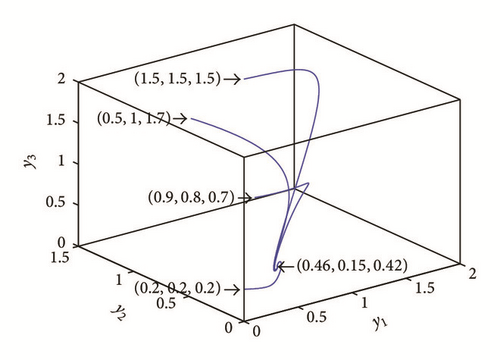
Clearly, Figure 1 shows the asymptotic approach of the solutions, which started from different initial points to a positive equilibrium point (0.46, 0.15, 0.42), for the data given by (69). This confirms our obtained result regarding the existence of globally asymptotically stable positive point of system (3) provided that certain conditions hold.

Details are in the caption following the image — **Figure 1**
Open in figure viewer PowerPoint

3D phase plot of the system (3) for the data given by (69) starting from different initial values in which the solution approaches asymptotically to 0.46, 0.15, and 0.42.

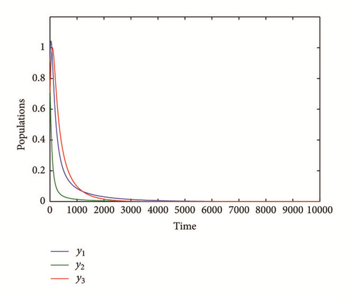
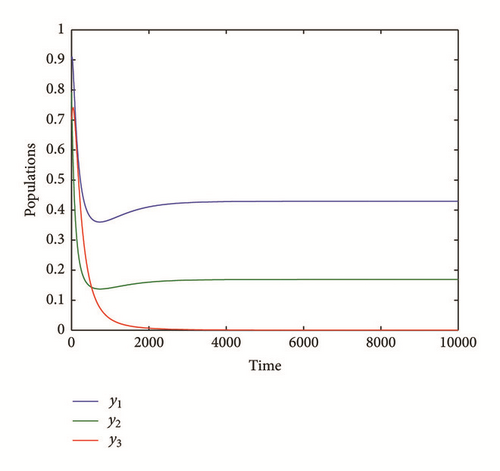
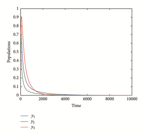
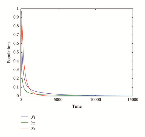
Now in order to discuss the effect of the parameters values of system (3) on the dynamical behavior of the system, the system is solved numerically for the data given in (69) with varying one parameter each time. It is observed that varying parameters values a₂, a₄, b₂, b₃, and b₄ have no qualitative effect on the dynamical behavior of system (3) and the system still approaches to a positive equilibrium point. On the other hand, when a₁ decreases in the range (a₁ ≤ 1.05) keeping other parameters fixed as given in (69) the dynamical behavior of system (3) approaches asymptotically to the vanished equilibrium point as shown in the typical figure given by Figure 2. Similar observations have been obtained on the behavior of system (3) in case of increasing the parameter a₃ in the range (a₃ ≥ 0.8) or decreasing the parameter b₁ in the range (b₁ ≤ 0.2), with keeping other parameters fixed as given in (69), and then the solution of system (3) is depicted in Figures 3 and 4, respectively. Finally, for the parameters a₂ = 0.9 and b₄ = 0.7 with other parameters fixed as given in (69), the solution of system (3) approaches asymptotically to the predator free equilibrium point as shown in the Figure 5.

7. Discussion

In this paper, a model that describes the prey-predator system having a refuge and stage structure properties in the prey population has been proposed and studied analytically as well as numerically. Sufficient conditions which ensure the stability of equilibria and the existence of local bifurcation are obtained. The effect of each parameter on the dynamical behavior of system (3) is studied numerically and the trajectories of the system are drowned in the typical figures. According to these figures, which represent the solution of system (3) for the data given by (69), the following conclusions are obtained.

(1)
System (3) has no periodic dynamics rather than the fact that the system approaches asymptotically to one of their equilibrium points depending on the set of parameter data and the stability conditions that are satisfied.
(2)
Although the position of the positive equilibrium point in the interior of changed as varying in the parameters values a₂, a₄, b₂, b₃, and b₄, there is no qualitative change in the dynamical behavior of system (3) and the system still approaches to a positive equilibrium point. Accordingly adding the refuge factor which is included implicitly in these parameters plays a vital role in the stabilizing of the system at the positive equilibrium point.
(3)
Decreasing in the value of growth rate of immature prey or in the value of conversion rate from immature prey to mature prey keeping the rest of parameter as in (69) leads to destabilizing of the positive equilibrium point and the system approaches asymptotically to the vanishing equilibrium point, which means losing the persistence of system (3).
(4)
Increasing in the value of grownup rate of immature prey keeping the rest of parameter as in (69) leads to destabilizing of the positive equilibrium point and the system approaches asymptotically to the vanishing equilibrium point too, which means losing the persistence of system (3).
(5)
Finally, for the data given by (69), increasing intraspecific competition of immature prey and natural death rate of the predator leads to destabilizing of the positive equilibrium point and the solution approaches instead asymptotically to the predator free equilibrium point, which confirm our obtained analytical results represented by conditions (21)-(22).

Competing Interests

The authors declare that they have no competing interests.

References

1 Freedman H. I., Deterministic Mathematical Models in Population Ecology, 1980, 57, Marcel Dekker, New York, NY, USA, MR586941.
Google Scholar
2 Murray J. D., Mathematical Biology, 2002, 3rd edition, Springer, Berlin, Germany.
10.1007/b98868
Google Scholar
3 Dubey B. and Upadhyay R. K., Persistence and extinction of one-prey and two-predator system, Nonlinear Analysis: Modelling and Control. (2004) 9, no. 4, 307–329.
10.15388/NA.2004.9.4.15147
Google Scholar
4 Gakkhar S., Singh B., and Naji R. K., Dynamical behavior of two predators competing over a single prey, BioSystems. (2007) 90, no. 3, 808–817, https://doi.org/10.1016/j.biosystems.2007.04.003, 2-s2.0-35648932486.
10.1016/j.biosystems.2007.04.003
PubMed Web of Science® Google Scholar
5 Kar T. K. and Batabyal A., Persistence and stability of a two prey one predator, International Journal of Engineering, Science and Technology. (2010) 2, no. 2, 174–190.
10.4314/ijest.v2i2.59164
Google Scholar
6 Samanta G. P., Analysis of a delay nonautonomous predator-prey system with disease in the prey, Nonlinear Analysis: Modelling and Control. (2010) 15, no. 1, 97–108, Zbl1217.93073.
10.15388/NA.2010.15.1.14367
Web of Science® Google Scholar
7 Wang W. and Chen L., A predator-prey system with stage-structure for predator, Computers and Mathematics with Applications. (1997) 33, no. 8, 83–91, 2-s2.0-0031124171.
10.1016/S0898-1221(97)00056-4
Web of Science® Google Scholar
8 Bernard O. and Souissi S., Qualitative behavior of stage-structured populations: application to structural validation, Journal of Mathematical Biology. (1998) 37, no. 4, 291–308, https://doi.org/10.1007/s002850050130, MR1651631, 2-s2.0-0000927270.
10.1007/s002850050130
Web of Science® Google Scholar
9 Zhang X., Chen L., and Neumann A. U., The stage-structured predator-prey model and optimal harvesting policy, Mathematical Biosciences. (2000) 168, no. 2, 201–210, https://doi.org/10.1016/s0025-5564(00)00033-x, MR1802141, 2-s2.0-0033668215.
10.1016/S0025-5564(00)00033-X
CAS PubMed Web of Science® Google Scholar
10 Cui J., Chen L., and Wang W., The effect of dispersal on population growth with stage-structure, Computers and Mathematics with Applications. (2000) 39, no. 1-2, 91–102, 2-s2.0-0012099291.
10.1016/S0898-1221(99)00316-8
Web of Science® Google Scholar
11 Cui J. and Takeuchi Y., A predator-prey system with a stage structure for the prey, Mathematical and Computer Modelling. (2006) 44, no. 11-12, 1126–1132, https://doi.org/10.1016/j.mcm.2006.04.001, MR2256954, 2-s2.0-33746907779.
10.1016/j.mcm.2006.04.001
Google Scholar
12 Liu S. and Beretta E., A stage-structured predator-prey model of Beddington-DeAngelis type, SIAM Journal on Applied Mathematics. (2006) 66, no. 4, 1101–1129, https://doi.org/10.1137/050630003, MR2246048, 2-s2.0-33747198005.
10.1137/050630003
Web of Science® Google Scholar
13 Xu S., Dynamics of a general prey-predator model with prey-stage structure and diffusive effects, Computers and Mathematics with Applications. (2014) 68, no. 3, 405–423, https://doi.org/10.1016/j.camwa.2014.06.016, 2-s2.0-84904669151.
10.1016/j.camwa.2014.06.016
Web of Science® Google Scholar
14 González-Olivares E. and Ramos-Jiliberto R., Dynamic consequences of prey refuges in a simple model system: more prey, fewer predators and enhanced stability, Ecological Modelling. (2003) 166, no. 1-2, 135–146, https://doi.org/10.1016/s0304-3800(03)00131-5, 2-s2.0-0348077455.
10.1016/S0304-3800(03)00131-5
Web of Science® Google Scholar
15 Kar T. K., Stability analysis of a prey-predator model incorporating a prey refuge, Communications in Nonlinear Science and Numerical Simulation. (2005) 10, no. 6, 681–691, https://doi.org/10.1016/j.cnsns.2003.08.006, MR2121754, 2-s2.0-11144275393.
10.1016/j.cnsns.2003.08.006
Google Scholar
16 Huang Y., Chen F., and Zhong L., Stability analysis of a prey-predator model with Holling type III response function incorporating a prey refuge, Applied Mathematics and Computation. (2006) 182, no. 1, 672–683, https://doi.org/10.1016/j.amc.2006.04.030, MR2292077, 2-s2.0-33750824327.
10.1016/j.amc.2006.04.030
Web of Science® Google Scholar
17 Ma Z., Li W., Zhao Y., Wang W., Zhang H., and Li Z., Effects of prey refuges on a predator-prey model with a class of functional responses: the role of refuges, Mathematical Biosciences. (2009) 218, no. 2, 73–79, 19167411, https://doi.org/10.1016/j.mbs.2008.12.008, MR2513672, 2-s2.0-62249093792, 19167411.
10.1016/j.mbs.2008.12.008
PubMed Web of Science® Google Scholar
18 Křivan V., On the Gause predator-prey model with a refuge: a fresh look at the history, Journal of Theoretical Biology. (2011) 274, no. 1, 67–73, https://doi.org/10.1016/j.jtbi.2011.01.016, MR2974938, 2-s2.0-79251592857.
10.1016/j.jtbi.2011.01.016
PubMed Web of Science® Google Scholar
19 Wang S. and Ma Z., Analysis of an ecoepidemiological model with prey refuges, Journal of Applied Mathematics. (2012) 2012, 16, 371685, https://doi.org/10.1155/2012/371685, 2-s2.0-84871399400.
10.1155/2012/371685
Google Scholar
20 Pal A. K. and Samanta G. P., A ratio-dependent eco-epidemiological model incorporating a prey refuge, Universal Journal of Applied Mathematics. (2013) 1, no. 2, 86–100.
10.13189/ujam.2013.010208
Google Scholar
21 De Rossi A., Ferrua I., Perracchione E., Ruatta G., and Venturino E., Competition models with niche for squirrel population dynamics, 1558, Proceedings of the 11th International Conference of Numerical Analysis and Applied Mathematics( ICNAAM ′13), September 2013, Rhodes, Greece, 1818–1821, AIP Conference Proceedings, https://doi.org/10.1063/1.4825880.
10.1063/1.4825880
Google Scholar
22 Haque M., Rahman M. S., Venturino E., and Li B.-L., Effect of a functional response-dependent prey refuge in a predator-prey model, Ecological Complexity. (2014) 20, 248–256, https://doi.org/10.1016/j.ecocom.2014.04.001, 2-s2.0-84918573387.
10.1016/j.ecocom.2014.04.001
Web of Science® Google Scholar
23 Cavoretto R., De Rossi A., Perracchione E., and Venturino E., Reliable approximation of separatrix manifolds in competition models with safety niches, International Journal of Computer Mathematics. (2015) 92, no. 9, 1826–1837, https://doi.org/10.1080/00207160.2013.867955, MR3356224, 2-s2.0-84896574146.
10.1080/00207160.2013.867955
Web of Science® Google Scholar
24 Perko L., Differential Equations and Dynamical Systems, 2001, 7, 3rd edition, Springer, New York, NY, USA, https://doi.org/10.1007/978-1-4613-0003-8, MR1801796.
10.1007/978-1-4613-0003-8
Google Scholar

Citing Literature

All articles

The Dynamical Analysis of a Prey-Predator Model with a Refuge-Stage Structure Prey Population

Abstract

1. Introduction

2. Mathematical Model

3. Local Stability Analysis

4. Global Stability

5. Local Bifurcation

6. Numerical Simulations

7. Discussion

Competing Interests

References

Citing Literature

Figures

References

Information

About Wiley Online Library

Help & Support

Opportunities

Connect with Wiley

The Dynamical Analysis of a Prey-Predator Model with a Refuge-Stage Structure Prey Population

Abstract

1. Introduction

2. Mathematical Model

3. Local Stability Analysis

4. Global Stability

5. Local Bifurcation

6. Numerical Simulations

7. Discussion

Competing Interests

References

Citing Literature

Figures

References

Related

Information