Catchment hydrologic cycle takes on different patterns across temporal scales. The interim between event-scale hydrologic process and mean annual water-energy correlation pattern requires further examination to justify self-consistent understanding. In this paper, the temporal scale transition revealed by observation and simulation was evaluated in an information theoretical framework named Aleatory Epistemic Uncertainty Estimation. The Aleatory Uncertainty refers to posterior uncertainty of runoff given the input variables’ observations. The Epistemic Uncertainty refers to the posterior uncertainty increase due to the imperfect observation decoding in models. Daily hydrometeorological observations in 24 catchments were aggregated from 10 days to 1 year before implementing the information analysis. Estimations of information contents and flows of hydrologic terms across temporal scales were related with the catchments’ seasonality type. It also showed that information distilled by the monthly and annual water balance models applied here did not correspond to that provided by observations around temporal scale from two months to half a year. This calls for a better understanding of seasonal hydrologic mechanism.

1. Introduction

A major realm of hydrologic community is to figure out the components of hydrologic cycle. Each component should be determined either by observation or by an independent governing equation to guarantee the solvability of the problem. The accuracy of observation and domain of governing equations usually change with scales. The term scale here refers to the characteristic time (or length) of a process, observation, or model [1]. While large scale hydrologic patterns are expected to emerge by integrating detailed event-scale hydrologic control functions along the spatial and temporal paths, such reductionism approach often fails to distill the dominant factors that contribute to catchment’s long range hydrologic behaviours. On the other hand, the holism perspective has been widely adopted to provide coarse explanation of catchment’s mean annual water balance [2, 3]. A cut-through between the reductionism and holism paradigms is required for reaching a self-consistent understanding of hydrologic temporal scale transition [4].

One practical attempt toward this goal is to expand the existing mean annual models to fit for small temporal scale hydrologic simulation. Classical Budyko curve [5] which connects the ratio of catchment’s actual evapotranspiration (E) to precipitation (P) and dryness index (PE/P, where PE denotes potential evapotranspiration) can not exert first-order control of water balance for excluding the impact of soil moisture change within the scales the model focuses on [6–8]. By including the soil moisture storage term (S), the expanded models could be applied for seasonal, even monthly, hydrologic simulation and prediction.

As is declared, the incorporation of new variable increases the system’s freedom degree, which should be compensated by introducing new independent governing equation. In Budyko curve, the water supply P is partitioned into actual evapotranspiration (E) and runoff (Q) with the evapotranspiration demand being PE. Accordingly, the adjusted models make a multistep precipitation partition given the water competition between catchment replenishment demand and evapotranspiration demand. Table 1 listed the analysis of some widely accepted water balance models following this cognitive framework.

Table 1. Structure analysis of water balance models¹.

Model	Replenishment demand	Evapotranspiration demand	Constitutive functions
ABCD [32]	b	PE
ABCD [32]	b	PE	E = ΔS × (1 − e^−PE/b)
DWBM [33]	S_max − S + PE	PE
DWBM [33]	S_max − S + PE	PE
TPWB [17]	SC	PE
TPWB [17]	SC	PE

¹Symbols without explicit explanation are model parameters.

Due to the same constraints of extreme zero-order and first-order boundary conditions where water supply far surpasses or falls behind demand, the curves above take on similar shapes and achieve similar satisfactory performances in monthly scale simulation. Each model requires 2 (in TPWB) to 4 (in ABCD or DWBM) parameters to adjust curve concavity and position to fit for observations. The statistic characteristics of state variables and parameters differ as the modelling scale changes [9]. It is interesting to make a closer examination of data-revealed hydrologic pattern and model performance during scale transition given the wide temporal scale gap between event-scale hydrologic process and annual-mean water balance.

Variables in large temporal scale hydrologic models are the aggregation of themselves in small scale models. The goal of these models is to find out the control of the aggregated variables on that period’s total water balance, which is determined by the inner-scale temporal distribution of hydrologic events and catchment’s storage capacity [10]. For instance, given the same average water and energy supply, catchments with uniformly distributed rainfall and large storage capacity tend to generate less direct runoff and more evapotranspiration. These determinants are simplified as state variable S in the water balance models. The motivation of this paper was to quantify data-revealed (potential) and model-revealed (achieved) control of hydrometeorological variables’ mean values on catchments average water balance over different temporal scales. The estimations were implemented within an information theoretical framework named Aleatory Epistemic Uncertainty Estimation (AEUE) [11] for its mathematical elegance in assessing such insufficient information control problems.

The rest of the paper is structured as follows: in Section 2, the definitions and properties of AEUE are briefly introduced before clarifying its logical extensions and technical adaptions in this work. Section 3 gives the data description. The results and their interpretations are in Sections 4 and 5. The last section draws conclusion and recommends directions for future work.

2. Methodology

2.1. Aleatory and Epistemic Uncertainty in Hydrologic Simulation

It is intuitively believed that infrequent samples of a random variable bring more surprise or information. The mathematical expression of this common sense is that information provided by an observation should be a decreasing function of its probability. If we further require the additive property of information between independent events, the form of information content attributed to a sample with probability p should be −log⁡p. The average information content of random variable X is

(1)

H(X) and h(X) are defined as discrete and continuous Shannon entropy [12], both measured in bits for logarithm base 2. The two terms are connected with the following limitation relation [13]:

(2)

As is shown in Figure 1, X^Δ denotes the discrete random variable by scattering the continuous random variable X into bins with width of Δ in its probability density function (p.d.f.). h(X) − log⁡Δ represents the information content required to describe X to −log⁡Δ bit accuracy [13]. Here −log⁡Δ bit accuracy means X takes the same value in a Δ width bin in the p.d.f. curve.

Details are in the caption following the image — **Figure 1**
Open in figure viewer PowerPoint

Quantization of continuous random variable.

Entropy maps the probability distribution function to a real number. Apply this functional map to both sides of Bayes’ Theorem; we have

(3)

(4)

In the literature of information theory, they are denoted as

(5)

(6)

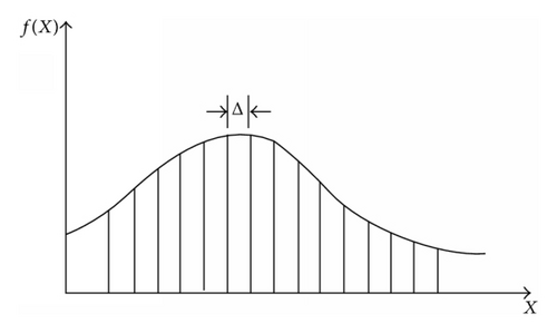
Each term in the equations above is named in correspondence with that in Bayes’ Theorem. Explicitly, H(X∣Y) and h(X∣Y) are called conditional entropy, which represent the posterior uncertainty of X given the knowledge of Y. H(X) and h(X) represent the prior uncertainty. I(X; Y) is called mutual information. It represents the information contribution one variable provides to the other.

The application of Bayes’ Theorem in hydrologic simulation assessment [14–16] endows each of the information terms with its hydrologic significance. Conceive X as the hydrologic variable to be simulated and Y as the input variable observations, both taken as continuous random variables; (6) quantifies the residual uncertainty of the hydrologic system given the inaccurate and insufficient observation system. This uncertainty is named as Aleatory Uncertainty (AU) [11]:

(7)

Here X_o, X_i represent the observed output and input random variables of hydrologic models. It should be noted that X_i is usually high dimensional, since information comes from different resources (both hydrometeorology and underlying surface observations) and lagging effects of former hydrologic behaviours. Models try to distill the largest information from X_i to construct their simulations X_s. Given that X_s is function of X_i, Data Processing Inequality Theorem [13] confirms that the potential maximum information models could distill (represented as I(X_o, X_s)) is not larger than that provided by the original data (represented as I(X_o, X_i)). A detailed proof is given in Appendix. The information loss due to imperfect input data processing is defined as Epistemic Uncertainty (EU) [11]:

(8)

Equations (7) and (8) construct the Aleatory Epistemic Uncertainty Estimation (AEUE) framework. The sum of AU and EU is the posterior uncertainty of the hydrologic system given the simulation system.

2.2. Extending AEUE for Temporal Scale Information Analysis

To implement AEUE across temporal scales, daily hydrometeorologic observations were aggregated into different temporal scales. The aggregated data were used for estimation of each term in (7) and (8). To achieve a more explicit information analysis, we adapted the strategy to gradually expand input variable species and lagging steps to detect the decreasing trajectory of AU. The decrease is attributed as the information contribution of the included variables. For example, AU(Q; P, PE) − AU(Q; P) (which simplified to I(Q; P, PE) − I(Q; P) according to (7)) represents the information contribution of including energy supply constraints (PE) in simulation, while AU(Q; P, P_former, PE, PE_former) − AU(Q; P, PE) (which simplified to I(Q; P, P_former, PE, PE_former) − I(Q; P, PE)) represents the information contribution of former calculating steps’ hydrologic lagging effects; in other words, it denotes the soil moisture memory significance.

EU of two typical water balance models were estimated. The Two-Parameter Water Balance (TPWB) Model [17] was preferred for its simplicity and satisfactory performance at monthly scale. The model structure was listed in Table 1. The other model was Budyko Model. It is the combination of Budyko curve [18] and mass conservation function. The most significant distinction between the two models is that TPWB adapts iterative structure. The performance of iterative models depends on its state variable’s capacity to distill information of system’s lagging effects and its constitutive functions’ capacity to utilize the distilled information. These two factors were discerned through distinguishing I(Q; P, P_former, PE, PE_former), I(Q; P, PE, S), and I(Q; Q_s), where S represents model’s state variable and Q_s represents simulated runoff. The difference of the first two terms tells state variable’s representativeness and difference between the last two terms tells constitutive function’s data processing efficiency.

Given the analysis above, the explicit AEUE framework estimates the terms as listed in Table 2.

Table 2. Information terms to be estimated.

Classification	Estimated terms
Observation	h(Q)
Focused	I(Q; P), I(Q; P, P_former)
	I(Q; P, PE), I(Q; P, P_former, PE, PE_former)
	I(Q; P, P_former, PE, PE_former, Q_former)
Model	TPWB: I(Q; Q_s), I(Q; P, PE, S)
Focused	Budyko: I(Q; Q_s)

2.3. High Dimensional Mutual Information Estimator

The major obstacle AEUE faces is the estimation of high dimensional mutual information terms in Table 2. Samples of finite length can not support accurate estimation of their probability distribution in high dimensional spaces. This phenomenon, known as dimensionality curse [19], has hindered the definition-based estimation of mutual information. Given this, some “nonplugin” methods have been developed. The basic idea is to construct relation between carefully designed sample statistics with its entropy [20] or to perform transform for a step-by-step entropy estimation [21]. Mutual information was estimated afterwards with the following equation:

(9)

As can be detected, error may accumulate in these algorithms.

The estimator we adapted here belongs to the first mode but makes direct estimation of mutual information. The formula is based on the concept of k nearest neighbour distances [22]:

(10)

Here ψ(x) is the digamma function, ψ(x) = Γ(x) ⁻¹dΓ(x)/dx. k is order of nearest neighbour; n_x(i) and n_y(i) are the numbers of samples that are within the kth nearest crisscross surrounding sample point i. k takes 4 to balance the statistical error and systematic error according to Kraskov’s suggestion [22].

An intuitive explanation of (10) is that it estimates mutual information with statistics that depicts the average concentrating density of each window opened around a sample point. Numerical experiments showed that even less than 30 sample size produces satisfying results. For a strict proof, please refer to Kraskov et al. [22].

The samples’ distance function should be predefined to determine n_x and n_y in (10). Since different dimensions hold specific hydrologic meanings and are not symmetric, the distance could not be efficiently depicted with Euclidean norm. Kernel trick was adapted to implicitly measure sample distances in their feature space. Kernels were chosen by optimizing their correspondent support vector regression (SVR) [23] performance implemented on the test set. Satisfactory kernel SVR performance suggests well-balanced compromise between minimizing variance and bias in the proper feature space. Results showed that kernel SVR was effective in performing high dimensional regression of hydrologic variables [24–28]. The following function was used to depict the distance between two input variable samples x₁ and x₂:

(11)

f(x) is the support vector regression function that fitted the input to the output variable. n_x and n_y were determined after the calculation of distances between samples.

In practice, the support vector regression was implemented using the LIBSVM package [29]. Radial basic function kernel was adopted for its satisfying performance. The data were first normalized to [−1,1] to balance the impact of different dimensional terms. Results were sensitive to the penalty function parameter c and kernel parameter g, both of which were autocalibrated with particle swarm optimization algorithm [30].

3. Data

24 catchments with daily hydrologic records (including P, PE, and Q) from MOPEX data set [31] were selected to implement cross temporal scale information analysis. Given their temporal water-energy distribution patterns, the selected catchments are classified into 4 groups, explicitly, weak seasonality with synchronous rainfall energy distribution (WS), weak seasonality with asynchronous rainfall energy distribution (WA), strong seasonality with synchronous rainfall energy distribution (SS), and strong seasonality with asynchronous rainfall energy climate (SA). The classification standard was based on the amplitude and phase of the average daily rainfall fitted with sine curve. If the amplitude was less than 0.45, the catchment was taken as weak seasonality. If the phase of rainfall was inverse to that of potential evapotranspiration, it was taken as asynchronous rainfall energy climate type. The general conditions of the catchments were listed in Table 3. The vegetation, soil type, land use, and other specific catchment information are available from the following link: ftp://hydrology.nws.noaa.gov/pub/gcip/mopex/US_Data/.

Table 3. Catchment condition.

Climate type	ID	Location	Area (km²)	P_mean (mm)	PE_mean (mm)	Q_mean (mm)
WA	02143000	81°W, 36°N	215	1299	882	553
	02165000	82°W, 34°N	611	1252	965	539
	02329000	84°W, 31°N	2953	1321	1101	330
	02375500	87°W, 31°N	9886	1452	1061	549
	02478500	86°W, 31°N	6967	1440	1055	489

WS	05585000	91°W, 40°N	3349	922	993	232
	06908000	93°W, 39°N	2901	1001	1066	261
	07019000	91°W, 38°N	9811	1006	959	303
	07177500	96°W, 36°N	2344	948	1259	221
	07243500	96°W, 36°N	5227	935	1303	160

SA	02414500	86°W, 33°N	4338	1371	976	542
	02472000	89°W, 31°N	1924	1442	1059	509
	11025500	117°W, 33°N	290	522	1407	34
	11532500	124°W, 42°N	1577	2748	751	2212
	12459000	121°W, 48°N	2590	1613	681	1105
	13337000	116°W, 46°N	3056	1287	775	872
	14359000	123°W, 42°N	5317	1052	851	510

SS	05418500	91°W, 42°N	4022	854	1017	254
	05454500	91°W, 41°N	8472	839	984	224
	05484500	94°W, 41°N	8912	794	998	117
	06810000	96°W, 40°N	7268	808	1027	173
	06892000	95°W, 39°N	1052	941	1110	228
	06914000	95°W, 38°N	865	950	1186	236
	07183000	96°W, 37°N	9889	877	1250	187

4. Aleatory and Epistemic Uncertainty across Temporal Scales

4.1. Aleatory Uncertainty

Considering the implication of (2), the Aleatory Uncertainty comparison across temporal scales requires a scheme to preset resolution for each temporal scale. Since the acceptable deviation of small temporal scale hydrologic models should be stricter than larger scale models, we prerequired relative constant resolution across temporal scales. Explicitly, the width of the bin into which the objective variable is clustered in the p.d.f. curve is proportional to its mean value. It was further assumed that the mean value is proportional to its temporal scales. Thus, the quantization correction term in (2) is proportional to the logarithm of the temporal scale. For two scales m and n into which daily runoff observation data were aggregated, the entropy difference for depicting them with specific resolutions is

(12)

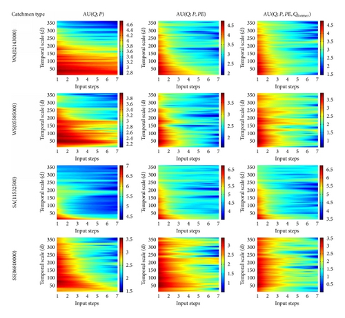
Given this baseline, the estimated Aleatory Uncertainty was shown as follows.

In each subgraph above, the abscissa represents the input steps; for example, number n denotes that the current and (n − 1) lagging steps’ input observations were used to decrease the uncertainty of runoff estimation. The ordinate represents the estimating temporal scale, which varied from 10 days to a year.

The general pattern is that AU decreases as temporal scale expands or more lagging input observations were included. It could be depicted that AU was closely related to catchment’s seasonality type; specifically

(13)

The detailed analysis discerning each term’s information contribution for different catchments was discussed in the next session.

4.2. Epistemic Uncertainty

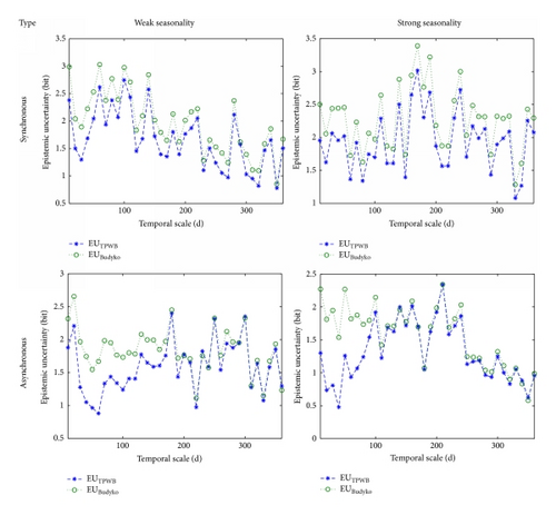
The estimated Epistemic Uncertainty across temporal scales was shown in Figure 3.

For TPWB model, maximum EU appears around temporal scales from 2 months to half a year. This showed that, at seasonal temporal scale, the model can not distill the information provided by the data effectively.

The EU difference between TPWB and Budyko Model was related to the catchment’s seasonality. In 11 out of 14 asynchronous seasonality catchments, EU differs significantly at small temporal scales. The difference diminished as scale expands. In the remaining 3 asynchronous catchments and 14 synchronous catchments, the difference stayed relatively constant across temporal scales.

5. Specific Information Analysis

5.1. Information Contribution of Included Input Terms

The including of new information sources could decrease simulation uncertainty. The specific information contribution of including energy provision PE and observed previous runoff Q_p was obtained by subtracting the right column graphs from the left column ones (Figure 4). For instance, AU(Q; P) − AU(Q; P, PE) denotes the information contribution of considering PE in the simulation.

For all the 10 weak seasonality catchments and 5 out of 14 strong seasonality catchments, the information contribution of PE was more significant at temporal scales of less than half a year. It was distributed more uniformly across temporal scales in the 9 left strong seasonality catchments.

The prominent information contribution of previous runoff at small scales in some catchments was attributed to runoff convergence influence.

5.2. Information Contribution of Soil Moisture Memory

Previous hydrologic behaviour exerts influence on current hydrologic response due to the storage capacity of soil moisture. Here this influence is defined as soil moisture memory and was represented by the difference between splines in each subgraph of Figure 2.

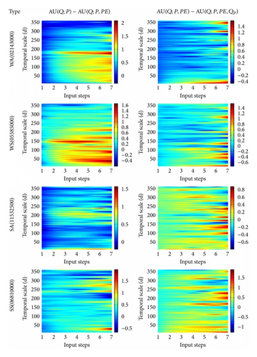
The second dissection scheme checks the information contribution of including lagged inputs in mutual information estimation. This is implemented by making differences in mutual information estimated with different input steps; for instance, the nth spline in each graph from Figure 5 equals the difference of the (n + 1)th spline and nth spline in the corresponding graph from Figure 6.

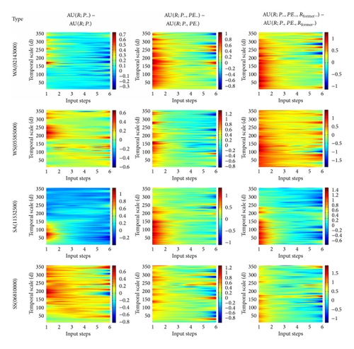
It could be depicted that the first lagging steps’ input variables provide most information contribution across all the temporal scales estimated here. As shown in the first column of Figure 5, these lagging effects were not significant when considering only the water provision. The consideration of energy provision is of key importance in estimating the soil moisture length.

5.3. Dissection of Model’s Information Distilling Capacity

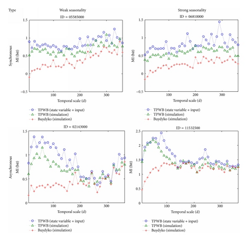
As was declared, the simulation capacity of iterative structure models depends on their capacity to distill lagging effects information and process such information. The information distilling and processing capacity were discerned in the following graphs.

The ordinate of each graph denotes mutual information. I(Q; I_c, S) represents the mutual information between runoff and current input together with current state variable. It denotes model’s capacity to distill lagging effects from previous hydrologic behaviours. The difference between I(Q; I_c, S) and I(Q; Q_s) denotes model’s capacity to process the information it distilled.

It could be depicted that, in synchronous climate catchments, the information distilled by TPWB and Budyko Model increases as temporal scale expands, while, in asynchronous climate catchments, the information distilling capacity of TPWB does not change monotonously with temporal scales.

6. Discussion and Conclusion

The aggregation of event-scale hydrologic processes yields to the large temporal scale water-energy correlation pattern. The temporal scale transition was examined in the extended Aleatory Epistemic Uncertainty Estimation framework.

The Aleatory Uncertainty quantified the uncertainty caused by inaccurate and insufficient observation. For a large temporal scale, since the daily observations were aggregated, the large number law guaranteed that the accumulated error tended to 0 when there was no systematic observation bias. Thus, AU was mainly attributed to the insufficience of data. The aggregated variables could exert certain control on the total water balance. The control significance was closely related to the seasonality type as quantified in the previous session.

The Epistemic Uncertainty of a monthly and mean annual water balance model was estimated. The performance of TPWB was evaluated by quantifying its information distilling capacity and data processing efficiency. Results showed that information distilled by the models applied here did not correspond to the information provided by input observations around temporal scale from two months to half a year. This called for a better understanding of seasonal hydrologic mechanism. The information distilling capacity difference of TPWB and Budyko Model was related to the inner-year distribution of water and energy. In asynchronous catchments, the difference converged to 0 at half year scale, which suggested close hydrologic cycle.

The evaluations also revealed some counterintuitive phenomenon that needs to be stressed and explained. The meaning of soil storage capacity from a large temporal scale perspective was not as physically clear as it is in event scale. The state variable S is influenced by the distribution of hydrologic processes and soil properties. The strict definition is required to explain the uncertainty differences in different seasonality catchments.

Conflict of Interests

The authors declare that there is no conflict of interests regarding the publication of this paper.

Acknowledgments

The authors are grateful to the financial supports offered by the National Science Foundation of China (51479088, 51179083, and 91225302). For detailed algorithm and estimation results, please refer to the following Github repository: https://github.com/emmore/Code/tree/master/My_Lib/Matlab_Lib. Finally, the authors should express their special thanks to Hoshin V. Gupta from University of Arizona for his insights and kindness.

Appendix

Data Processing Inequality

The Data Processing Inequality states that if X, Y, and Z form a Markov Chain (denoted as X → Y → Z), which means X and Z are conditionally independent given Y, then

(A.1)

The proof is given due to the nonnegative effects of information:

(A.2)

Specifically, if Z = f(Y), then X → Y → f(Y); we have

(A.3)

This confirms that information could not be produced through data processing.

For hydrologic simulation, due to the nonnegative effects of information, the inclusion of new input terms will not increase AU in our context. From a functional perspective, models act as a function that transfers input variables into output variables, with the estimated state variables as intermediate products. Variables from models form the following Markov Chain:

(A.4)

This clarified the reason to perform model information diagnosis as presented in Figure 6.

References

1 Bloschl G. and Sivapalan M., Scale issues in hydrological modelling: a review, Hydrological Processes. (1995) 9, no. 3-4, 251–290, https://doi.org/10.1002/hyp.3360090305, 2-s2.0-0029413274.
10.1002/hyp.3360090305
Web of Science® Google Scholar
2 Zhang L., Dawes W. R., and Walker G. R., Response of mean annual evapotranspiration to vegetation changes at catchment scale, Water Resources Research. (2001) 37, no. 3, 701–708, https://doi.org/10.1029/2000wr900325, 2-s2.0-0034987502.
10.1029/2000WR900325
Web of Science® Google Scholar
3 Yang D., Sun F., Liu Z., Cong Z., Ni G., and Lei Z., Analyzing spatial and temporal variability of annual water-energy balance in nonhumid regions of China using the budyko hypothesis, Water Resources Research. (2007) 43, no. 4, W04426, https://doi.org/10.1029/2006wr005224, 2-s2.0-34249047694.
10.1029/2006WR005224
Web of Science® Google Scholar
4 Wang D. and Tang Y. A., A one-parameter Budyko model for water balance captures emergent behavior in darwinian hydrologic models, Geophysical Research Letters. (2014) 41, no. 13, 4569–4577, https://doi.org/10.1002/2014gl060509, 2-s2.0-84903429076.
10.1002/2014GL060509
Web of Science® Google Scholar
5 Budyko M. I., The heat balance of the earth′s surface, Soviet Geography. (1961) 2, no. 4, 3–13, https://doi.org/10.1080/00385417.1961.10770761.
10.1080/00385417.1961.10770761
Google Scholar
6 Sankarasubramanian A. and Vogel R. M., Annual hydroclimatology of the United States, Water Resources Research. (2002) 38, no. 6, 19-1–19-12, 2-s2.0-0036592345.
10.1029/2001WR000619
Web of Science® Google Scholar
7 Sankarasubramanian A. and Vogel R. M., Hydroclimatology of the continental United States, Geophysical Research Letters. (2003) 30, no. 7, article 1363, https://doi.org/10.1029/2002GL015937, 2-s2.0-0141539267.
10.1029/2002GL015937
Web of Science® Google Scholar
8 Tekleab S., Uhlenbrook S., Mohamed Y., Savenije H. H. G., Temesgen M., and Wenninger J., Water balance modeling of Upper Blue Nile catchments using a top-down approach, Hydrology and Earth System Sciences. (2011) 15, no. 7, 2179–2193, https://doi.org/10.5194/hess-15-2179-2011, 2-s2.0-79960364101.
10.5194/hess-15-2179-2011
Web of Science® Google Scholar
9 Hu Q., Wang Y., Liu K., and Wang Z., Monthly runoff simulation based on improved two-parameter monthly water volume balance model, Journal of Hohai University (Natural Sciences). (2007) 6.
Google Scholar
10 Porporato A., Daly E., and Rodriguez-Iturbe I., Soil water balance and ecosystem response to climate change, The American Naturalist. (2004) 164, no. 5, 625–632, https://doi.org/10.1086/424970, 2-s2.0-8744303901.
10.1086/424970
PubMed Web of Science® Google Scholar
11 Gong W., Gupta H. V., Yang D., Sricharan K., and HeroA. O.III, Estimating epistemic and aleatory uncertainties during hydrologic modeling: an information theoretic approach, Water Resources Research. (2013) 49, no. 4, 2253–2273, https://doi.org/10.1002/wrcr.20161, 2-s2.0-84877954935.
10.1002/wrcr.20161
Web of Science® Google Scholar
12 Shannon C. E., A mathematical theory of communication, ACM SIGMOBILE Mobile Computing and Communications Review. (1948) 5, no. 1, 3–55, Zbl1154.94303.
10.1145/584091.584093
Google Scholar
13 Cover T. M. and Thomas J. A., Elements of Information Theory, 2012, John Wiley & Sons, New York, NY, USA, MR2239987.
Google Scholar
14 Freer J., Beven K., and Ambroise B., Bayesian estimation of uncertainty in runoff prediction and the value of data: an application of the GLUE approach, Water Resources Research. (1996) 32, no. 7, 2161–2173, https://doi.org/10.1029/96wr03723, 2-s2.0-0029659801.
10.1029/95WR03723
Web of Science® Google Scholar
15 Kuczera G. and Parent E., Monte Carlo assessment of parameter uncertainty in conceptual catchment models: the metropolis algorithm, Journal of Hydrology. (1998) 211, no. 1, 69–85, https://doi.org/10.1016/s0022-1694(98)00198-x, 2-s2.0-0032214428.
10.1016/S0022-1694(98)00198-X
Web of Science® Google Scholar
16 Beven K. and Freer J., Equifinality, data assimilation, and uncertainty estimation in mechanistic modelling of complex environmental systems using the GLUE methodology, Journal of Hydrology. (2001) 249, no. 1–4, 11–29, https://doi.org/10.1016/s0022-1694(01)00421-8, 2-s2.0-0035426008.
10.1016/S0022-1694(01)00421-8
Web of Science® Google Scholar
17 Xiong L. and Guo S., A two-parameter monthly water balance model and its application, Journal of Hydrology. (1999) 216, no. 1-2, 111–123, https://doi.org/10.1016/s0022-1694(98)00297-2, 2-s2.0-0033535412.
10.1016/S0022-1694(98)00297-2
Web of Science® Google Scholar
18 Choudhury B. J., Evaluation of an empirical equation for annual evaporation using field observations and results from a biophysical model, Journal of Hydrology. (1999) 216, no. 1-2, 99–110, https://doi.org/10.1016/s0022-1694(98)00293-5, 2-s2.0-0033535419.
10.1016/S0022-1694(98)00293-5
Web of Science® Google Scholar
19 Bellman R. and Kalaba R., On adaptive control processes, IRE Transactions on Automatic Control. (1959) 4, no. 2, 1–9, https://doi.org/10.1109/tac.1959.1104847.
10.1109/TAC.1959.1104847
Google Scholar
20 Leonenko N., Pronzato L., and Savani V., A class of rényi information estimators for multidimensional densities, The Annals of Statistics. (2008) 36, no. 5, 2153–2182, https://doi.org/10.1214/07-aos539, MR2458183, 2-s2.0-54349103517.
10.1214/07-AOS539
Web of Science® Google Scholar
21 Gong W., Yang D., Gupta H. V., and Nearing G., Estimating information entropy for hydrological data: one-dimensional case, Water Resources Research. (2014) 50, no. 6, 5003–5018, https://doi.org/10.1002/2014wr015874, 2-s2.0-84902734475.
10.1002/2014WR015874
Web of Science® Google Scholar
22 Kraskov A., Stögbauer H., and Grassberger P., Estimating mutual information, Physical Review E. (2004) 69, no. 6, 066138, https://doi.org/10.1103/physreve.69.066138, MR2096503.
10.1103/PhysRevE.69.066138
CAS PubMed Web of Science® Google Scholar
23 Basak D., Pal S., and Patranabis D. C., Support vector regression, Neural Information Processing-Letters and Reviews. (2007) 11, no. 10, 203–224.
Google Scholar
24 Dibike Y. B., Velickov S., Solomatine D., and Abbott M. B., Model induction with support vector machines: introduction and applications, Journal of Computing in Civil Engineering. (2001) 15, no. 3, 208–216, https://doi.org/10.1061/(asce)0887-3801(2001)15:3(208), 2-s2.0-0035398081.
10.1061/(ASCE)0887-3801(2001)15:3(208)
Web of Science® Google Scholar
25 Asefa T., Kemblowski M., McKee M., and Khalil A., Multi-time scale stream flow predictions: the support vector machines approach, Journal of Hydrology. (2006) 318, no. 1–4, 7–16, https://doi.org/10.1016/j.jhydrol.2005.06.001, 2-s2.0-31044438334.
10.1016/j.jhydrol.2005.06.001
Web of Science® Google Scholar
26 Behzad M., Asghari K., Eazi M., and Palhang M., Generalization performance of support vector machines and neural networks in runoff modeling, Expert Systems with Applications. (2009) 36, no. 4, 7624–7629, https://doi.org/10.1016/j.eswa.2008.09.053, 2-s2.0-60249084777.
10.1016/j.eswa.2008.09.053
Web of Science® Google Scholar
27 Gong W., Watershed model uncertainty analysis based on information entropy and mutual information [Ph.D. thesis], 2013, Department of Hydraulic Engineering, Tsinghua University, Beijing, China.
Google Scholar
28 Lin J.-Y., Cheng C.-T., and Chau K.-W., Using support vector machines for long-term discharge prediction, Hydrological Sciences Journal. (2006) 51, no. 4, 599–612, https://doi.org/10.1623/hysj.51.4.599, 2-s2.0-33746830757.
10.1623/hysj.51.4.599
Web of Science® Google Scholar
29 Chang C.-C. and Lin C.-J., LIBSVM: a library for support vector machines, ACM Transactions on Intelligent Systems and Technology. (2011) 2, no. 3, article 27, https://doi.org/10.1145/1961189.1961199, 2-s2.0-79955702502.
10.1145/1961189.1961199
Web of Science® Google Scholar
30 Shi Y. and Eberhart R., Modified particle swarm optimizer, Proceedings of the IEEE World Congress on Computational Intelligence Evolutionary Computation, May 1998, Anchorage, Alaska, USA, 69–73, https://doi.org/10.1109/ICEC.1998.699146, 2-s2.0-0031700696.
10.1109/ICEC.1998.699146
Google Scholar
31 Duan Q., Schaake J., Andréassian V., Franks S., Goteti G., Gupta H. V., Gusev Y. M., Habets F., Hall A., Hay L., Hogue T., Huang M., Leavesley G., Liang X., Nasonova O. N., Noilhan J., Oudin L., Sorooshian S., Wagener T., and Wood E. F., Model Parameter Estimation Experiment (MOPEX): an overview of science strategy and major results from the second and third workshops, Journal of Hydrology. (2006) 320, no. 1-2, 3–17, https://doi.org/10.1016/j.jhydrol.2005.07.031, 2-s2.0-33644551546.
10.1016/j.jhydrol.2005.07.031
Web of Science® Google Scholar
32 Thomas H. A., Improved methods for national water assessment, WR15249270A.
Google Scholar
33 Zhang L., Potter N., Hickel K., Zhang Y., and Shao Q., Water balance modeling over variable time scales based on the Budyko framework—model development and testing, Journal of Hydrology. (2008) 360, no. 1–4, 117–131, https://doi.org/10.1016/j.jhydrol.2008.07.021, 2-s2.0-51249096540.
10.1016/j.jhydrol.2008.07.021
Web of Science® Google Scholar

Citing Literature

All articles

Information Analysis of Catchment Hydrologic Patterns across Temporal Scales

Abstract

1. Introduction

2. Methodology

2.1. Aleatory and Epistemic Uncertainty in Hydrologic Simulation

2.2. Extending AEUE for Temporal Scale Information Analysis

2.3. High Dimensional Mutual Information Estimator

3. Data

4. Aleatory and Epistemic Uncertainty across Temporal Scales

4.1. Aleatory Uncertainty

4.2. Epistemic Uncertainty

5. Specific Information Analysis

5.1. Information Contribution of Included Input Terms

5.2. Information Contribution of Soil Moisture Memory

5.3. Dissection of Model’s Information Distilling Capacity

6. Discussion and Conclusion

Conflict of Interests

Acknowledgments

Appendix

Data Processing Inequality

References

Citing Literature

Figures

References

Information

About Wiley Online Library

Help & Support

Opportunities

Connect with Wiley

Information Analysis of Catchment Hydrologic Patterns across Temporal Scales

Abstract

1. Introduction

2. Methodology

2.1. Aleatory and Epistemic Uncertainty in Hydrologic Simulation

2.2. Extending AEUE for Temporal Scale Information Analysis

2.3. High Dimensional Mutual Information Estimator

3. Data

4. Aleatory and Epistemic Uncertainty across Temporal Scales

4.1. Aleatory Uncertainty

4.2. Epistemic Uncertainty

5. Specific Information Analysis

5.1. Information Contribution of Included Input Terms

5.2. Information Contribution of Soil Moisture Memory

5.3. Dissection of Model’s Information Distilling Capacity

6. Discussion and Conclusion

Conflict of Interests

Acknowledgments

Appendix

Data Processing Inequality

References

Citing Literature

Figures

References

Related

Information