Volume 2015, Issue 1 964824

Research Article

Open Access

Bayesian Estimation of Inequality and Poverty Indices in Case of Pareto Distribution Using Different Priors under LINEX Loss Function

Kamaljit Kaur,

Corresponding Author

Kamaljit Kaur

[email protected]

orcid.org/0000-0001-6736-1968

Department of Statistics, Panjab University, Chandigarh 160014, India puchd.ac.in

Search for more papers by this author

Sangeeta Arora,

Sangeeta Arora

Department of Statistics, Panjab University, Chandigarh 160014, India puchd.ac.in

Search for more papers by this author

Kalpana K. Mahajan,

Kalpana K. Mahajan

Department of Statistics, Panjab University, Chandigarh 160014, India puchd.ac.in

Search for more papers by this author

Kamaljit Kaur,

Corresponding Author

Kamaljit Kaur

[email protected]

orcid.org/0000-0001-6736-1968

Department of Statistics, Panjab University, Chandigarh 160014, India puchd.ac.in

Search for more papers by this author

Sangeeta Arora,

Sangeeta Arora

Department of Statistics, Panjab University, Chandigarh 160014, India puchd.ac.in

Search for more papers by this author

Kalpana K. Mahajan,

Kalpana K. Mahajan

Department of Statistics, Panjab University, Chandigarh 160014, India puchd.ac.in

Search for more papers by this author

First published: 29 January 2015

https://doi.org/10.1155/2015/964824

Citations: 3

Academic Editor: Karthik Devarajan

Share a link

Email
Wechat
Bluesky

Abstract

Bayesian estimators of Gini index and a Poverty measure are obtained in case of Pareto distribution under censored and complete setup. The said estimators are obtained using two noninformative priors, namely, uniform prior and Jeffreys’ prior, and one conjugate prior under the assumption of Linear Exponential (LINEX) loss function. Using simulation techniques, the relative efficiency of proposed estimators using different priors and loss functions is obtained. The performances of the proposed estimators have been compared on the basis of their simulated risks obtained under LINEX loss function.

1. Introduction

The Pareto distribution is a skewed, heavy-tailed distribution that is used to model the distribution of incomes and other financial variables. It was introduced by Pareto [1] which has a probability density function of the form

()

and cumulative distribution function is

()

The parameter m in (2) represents the minimum income in the population under study and assumed to be known, while the other parameter α is assumed to be unknown.

The average income for Pareto distribution is

()

In the context of income inequality and poverty, Gini index and Poverty measure head count ratio are two most popular indices [2, 3]. Gini index is generally defined as

()

where

is the equation of the Lorenz curve and

is the mean of the distribution.

Equivalently, Gini index can also be defined as

()

where

is population Gini mean difference.

The Poverty index head count ratio P₀ is simply the count of the number of households whose incomes are below the poverty line divided by the total population. In terms of continuous distribution,

()

where, w₀(>m) is called Poverty Line.

In case of Pareto distribution, Gini index (G) [4, 5] is given by

()

and Poverty measure (P₀) is

()

where, w₀(>m) and λ₀ = (m/w₀).

Thus, w₀ is per capita annual income representing a minimum acceptable standard of living and P₀ represents the proportion of population having income equal to or less than w₀.

The estimation of Gini index (G) and Poverty measure (P₀) and the associated inference using classical approach (parametric and nonparametric) is available in literature [5–8]. However, in the Bayesian setup, this has not evoked the interest of many researchers [9, 10]. In the present paper, our focus will be on the estimation of inequality and poverty indices in the Bayesian setup.

When the Bayesian method is used, the choice of appropriate prior distribution plays an important role, which may be categorized as informative, noninformative, and conjugate priors [11, 12]. In the present paper, three priors (two noninformative priors and one conjugate prior) are used to estimate shape parameter, Gini index, Average income, and Poverty measure. The two noninformative priors are Uniform prior and Jeffreys’ prior, while conjugate prior is chosen as Truncated Erlang distribution.

In Bayesian estimation, the criterion for good estimators for the parameters of interest is the choice of appropriate loss function. In Bayesian estimation, two types of loss functions commonly used are Squared error loss function (SELF) and Linear exponential (LINEX) loss function. The simplest type of loss function is squared error, which is also referred to as quadratic loss is given as

()

where

is the estimator of θ.

The usual squared error loss function is symmetrical and associates equal importance to the losses due to overestimation and underestimation of equal magnitude. However, such a restriction may be impractical; for example, in estimation of shape parameter of Classical Pareto distribution, the overestimation and underestimation may not be of equal importance as over estimate of shape parameter gives an under-estimate of inequality index which seems to be more serious as compared to under estimate of shape parameter because we are often interested in reducing income inequality index. This leads one to think that an asymmetrical loss function be considered for estimation of shape parameter which associates greater importance to overestimation. A number of asymmetrical loss functions have been proposed in statistical literature [13–16]. Varian [16] proposed a useful asymmetrical loss function known as Linear exponential (LINEX) loss function which is given as

()

The posterior expectation of the LINEX loss function (10) is

()

where E(·) denotes posterior expectation with respect to the posterior density of θ.

By a result of Zellner [17] the Bayes estimator of θ denoted by

under the LINEX loss function is the value which minimizes posterior expectation and is given by

()

provided that the expectation E(e^−bθ) exists and is finite [18].

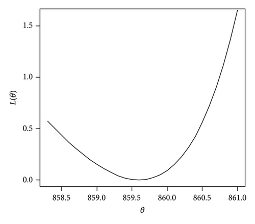
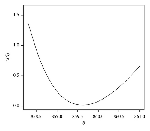
In Figures 1(a) and 1(b), values of L(θ) are plotted for the selected values of θ for b = 1 and b = −1. It is seen that, for b = 1, the function is quite asymmetric with a value exceeding the target being more serious than a value below the target. But, for b = −1, the function is also quite asymmetric with a value below the target value being more serious than a value exceeding the target.

Details are in the caption following the image — Open in figure viewer PowerPoint

For small value of b, the LINEX loss function can be expanded by Taylor’s series expansion as

()

Thus, the LINEX loss function is approximately equal to squared error loss function for small values of b (see Figure 1(c)).

This loss function has been considered by Zellner [17], Basu and Ebrahimi [19], and Afify [20] for different distributions.

In the present study, LINEX loss function is used for estimating the shape parameter, Gini index, Mean income, and a Poverty measure in the context of Pareto distribution using noninformative priors (Uniform prior and Jeffreys’ prior) and one conjugate prior (Truncated Erlang distribution) along with some assumptions regarding the sampled population. Bayesian approach with prior and posterior distributions along with sampling schemes in the context of Pareto distribution is given in Section 2. In Section 3, Bayesian estimators of shape parameter, Gini index, Mean income, and Poverty measure using different priors under the assumption of LINEX loss function are obtained. Finally, in Section 4, simulation is done to compare the efficiency of three different approaches using three priors and loss functions. The robustness of the hyperparameters is given in Section 4.1 through simulation study. Section 5 presents the conclusion of the study.

2. Preliminary about Sampling Scheme, Priors, and Posterior Densities

The Bayesian analysis of the Pareto distribution (2) is based on the following censored sampling scheme on personal income data. It is assumed that annual incomes of the n persons are under study but exact figures x₁, x₂, x₃, … , x_r are available only for those r individuals whose annual income does not exceed a prescribed annual income w₀(>m), and for the remaining (n − r) individuals, the exact income figures are unknown but we do know that their annual income exceed the prescribed figure w₀. Before the arrival of the sample data on personal incomes, n is predetermined but not r, which is a random. This censoring scheme used is referred as right censored sampling scheme.

The likelihood function L(α) for complete sample in case of Pareto distribution [4] is

()

In case of censored data, the likelihood function for any distribution [21] is

()

The likelihood function for Pareto distribution in censored sample is

()

where Z_w = ln⁡(m⁻ⁿP_w) is product income statistics [22] and

Bayes estimators of Gini index and Average income will not be convergent in the interval [0,1/2] and [0,1], respectively, and the method will fail to work. Hence, this difficulty is removed by assuming δ > 1, to obtain different Bayes estimators.

The prior and posterior densities for noninformative priors (Uniform prior and Jeffreys’ prior) and conjugate prior are explained below.

(i) Uniform Prior. In practice, the informative priors are not always available; for such situations, the use of noninformative priors is recommended. One of the most widely used noninformative prior, due to Laplace [23], is a uniform prior. Therefore, the uniform prior has been assumed for the estimation of the shape parameter of the Pareto distribution.

Uniform prior for α is

()

Combine likelihood function (16) with the prior density (17) by using Bayes theorem to obtain the posterior density as

()

where

is the upper incomplete gamma function and posterior density

is left truncated Gamma distribution.

(ii) Jeffreys’ Prior. Another noninformative prior has been suggested by Jeffreys [24] which is frequently used in situations where one does not have much information about the parameters. This is defined as the distribution of the parameters proportional to the square root of the determinants of the Fisher information matrix, that is,

, where I(α) = −E[(∂²/∂α²)log⁡L(α∣x)] is Fisher’s information of the given distribution. In case of Pareto distribution,

()

A motivation for Jeffreys’ prior is that Fisher’s information (I(α)) is an indicator of the amount of information brought by the model (observations) about α.

The posterior density is obtained as

()

which is left truncated Gamma distribution.

Note: Extension of Jeffreys’ Prior. Jeffreys’ prior is a particular case of extension of Jeffreys’ prior proposed by Al-Kutubi and Ibrahim [25], defined as

()

where c is a positive constant. For c = 0.5, it reduces to Jeffreys’ prior.

In case of Pareto distribution, this prior is

()

The posterior distribution by using extension to Jeffreys’ prior is obtained as

()

(iii) Conjugate Prior. The conjugate prior was introduced by Raiffa and Schlaifer [26], where the prior and posterior distributions are from the same family, that is, the form of the posterior density has the same distributional form as the prior distribution. For the existence of Gini index and Mean income for the Pareto distribution, we must take into account a truncated prior distribution since the random variable α is defined in (δ, ∞), where the constant δ > 1 is assumed to be known.

Let α have Truncated Erlang distribution [22]

()

where β and l are the hyperparameters.

The posterior density for α is

()

The posterior density

follows Truncated Erlang distribution with parameters (β + Z_w) and (r + l).

3. Bayesian Estimation under Linear Exponential (LINEX) Loss Function Using Different Priors

3.1. Bayesian Estimators Using Uniform Prior

Bayesian estimator

of α using uniform prior (17) and posterior density (18), under the assumption of the LINEX loss function (ref. (12)) is obtained as

()

Therefore,

()

The Bayes estimator

of G, using uniform prior is

()

(using formula (9) of 3.471, page 368 of Gradshteyn and Ryzhik [27]

, [Reβ > 0, Reγ > 0] where K_ν(·) is modified Bessel function of third kind).

Thereby,

()

The Bayes estimator

of M, using uniform prior is

()

(using formula (9) of 3.471, page 368 of Gradshteyn and Ryzhik [27]

, [Reβ > 0, Reγ > 0] where K_ν(·) is modified Bessel function of third kind)

()

The Bayes estimator

of P₀, using uniform prior, is

()

3.2. Bayesian Estimators Using Jeffreys’ Prior

In case of Jeffreys’ prior (19) and using posterior density (20), the Bayesian estimators of α, G, M, and P₀ under the assumption of the LINEX loss function are obtained as follows:

()

Note. The expression for extension of Jeffreys’ prior can be obtained with some modifications in Jeffreys’ prior and are listed below:

()

3.3. Bayesian Estimators Using Conjugate Prior

Using the Bayesian posterior density (25), the Bayes estimators of α, G, M, and P₀, under the assumption of the LINEX loss function are

()

Note: Case of Complete Sample. The Bayesian estimators for complete sample can be obtained using noninformative priors and conjugate prior by simply substituting r = n in the above estimators.

4. Simulation Study

In order to assess the statistical performance of these estimators of shape parameter, Gini index, Mean income, and Poverty measure using LINEX loss function, a simulation study is conduced. The estimated losses are computed using generated random samples from Pareto distribution of different sizes. These estimated losses are computed for sample sizes n = 20 (20) 100, α = 2.5 (1) 4.5, b = 1, δ = 1.5, and m = 450. The value of w₀ = 859.6 should be taken from Poverty line given by the Government of India in 2009-10 for urban people. For the conjugate prior, the values of hyperparameter are taken as β = 0.5, l = 2; β = 2, and l = 2. The estimated losses of α, G, M, and P₀ with LINEX loss function by using noninformative (Uniform prior and Jeffreys’ prior) and conjugate priors are tabulated in Tables 1, 2, 3, and 4, respectively.

1. Estimated loss functions for α using LINEX loss function.

n	α	Uniform prior	Jeffrey’s prior	Conjugate prior
n	α	Uniform prior	Jeffrey’s prior	β = 0.5 l = 2	β = 2 l = 2
20	2.5	0.200543	0.173893	0.112013	0.113299
	3.5	0.423936	0.357678	0.281125	0.371823
	4.5	0.719781	0.456351	0.311154	0.710794

40	2.5	0.110843	0.077269	0.050112	0.072872
	3.5	0.207535	0.204212	0.145707	0.174398
	4.5	0.324085	0.228739	0.207738	0.344289

60	2.5	0.065696	0.061891	0.058858	0.059336
	3.5	0.135812	0.104322	0.102511	0.123564
	4.5	0.283127	0.211419	0.149228	0.224148

80	2.5	0.048582	0.052477	0.044407	0.045243
	3.5	0.094729	0.094126	0.081215	0.089861
	4.5	0.146575	0.140906	0.126948	0.163061

100	2.5	0.047068	0.040324	0.034990	0.038336
	3.5	0.072414	0.071366	0.065080	0.070502
	4.5	0.112283	0.104459	0.099383	0.131260

2. Estimated loss functions for G using LINEX loss function.

n	α	Uniform prior	Jeffrey’s prior	Conjugate prior
n	α	Uniform prior	Jeffrey’s prior	β = 0.5 l = 2	β = 2 l = 2
20	2.5	0.003944	0.0031157	0.002672	0.057322
	3.5	0.000849	0.0007378	0.000700	0.016733
	4.5	0.000671	0.0005303	0.000463	0.009637

40	2.5	0.001503	0.0011873	0.000963	0.008362
	3.5	0.000642	0.0005590	0.000516	0.003782
	4.5	0.000314	0.0002975	0.000197	0.002782

60	2.5	0.000811	0.0007397	0.000692	0.006373
	3.5	0.000415	0.0003852	0.000319	0.001783
	4.5	0.000200	0.0001726	0.000159	0.000873

80	2.5	0.000687	0.0006286	0.000586	0.002637
	3.5	0.000298	0.0002746	0.000189	0.000978
	4.5	0.000141	0.0001403	0.000116	0.000512

100	2.5	0.000611	0.0005395	0.000483	0.001032
	3.5	0.000231	0.0002250	0.000102	0.000822
	4.5	0.000115	0.0001073	0.000083	0.000421

3. Estimated loss functions for M using LINEX loss function.

n	α	Uniform prior	Jeffrey’s prior	Conjugate prior
n	α	Uniform prior	Jeffrey’s prior	β = 0.5 l = 2	β = 2 l = 2
20	2.5	0.073957	0.0657402	0.026145	0.056465
	3.5	0.061835	0.0558135	0.015994	0.046743
	4.5	0.056649	0.0418561	0.012289	0.035673

40	2.5	0.073204	0.0555914	0.025888	0.043674
	3.5	0.060616	0.0466542	0.016802	0.040301
	4.5	0.055089	0.0435518	0.013802	0.031533

60	2.5	0.072393	0.0458580	0.026035	0.039373
	3.5	0.059386	0.0376830	0.017845	0.036373
	4.5	0.053528	0.0352241	0.015377	0.025377

80	2.5	0.071778	0.0360502	0.026361	0.030012
	3.5	0.058222	0.0286558	0.018818	0.029733
	4.5	0.051894	0.0267040	0.016845	0.020345

100	2.5	0.071070	0.0263228	0.020575	0.027973
	3.5	0.057185	0.0196096	0.019812	0.028732
	4.5	0.030343	0.0183061	0.018161	0.019637

4. Estimated loss functions for P₀ using LINEX loss function.

n	α	Uniform prior	Jeffrey’s prior	Conjugate prior
n	α	Uniform prior	Jeffrey’s prior	β = 0.5 l = 2	β = 2 l = 2
20	2.5	0.003918	0.0016639	0.0015042	0.0037360
	3.5	0.007714	0.0012619	0.0011718	0.0033510
	4.5	0.006892	0.0006375	0.0006100	0.0033324

40	2.5	0.003030	0.0012092	0.0011452	0.0013573
	3.5	0.001033	0.0007198	0.0007159	0.0016299
	4.5	0.001099	0.0003325	0.0003235	0.0011149

60	2.5	0.002237	0.0009517	0.0008915	0.0011249
	3.5	0.001652	0.0004774	0.0004483	0.0008925
	4.5	0.001019	0.0002165	0.0002040	0.0005813

80	2.5	0.001769	0.0007372	0.0007191	0.0009047
	3.5	0.001163	0.0003889	0.0003795	0.0006315
	4.5	0.000659	0.0001677	0.0001622	0.0003924

100	2.5	0.001009	0.0006512	0.0005704	0.0007186
	3.5	0.000465	0.0002854	0.0002770	0.0004269
	4.5	0.000287	0.0001354	0.0001240	0.0002843

It is observed from the above simulation study (ref. Tables 1, 2, 3, and 4) that

(i)
Bayesian estimators with conjugate prior (hyperparameter β = 0.5, l = 2) perform better as compared to noninformative priors as it has smaller estimated loss for α, G, M, and P₀;
(ii)
in case of noninformative priors, Jeffreys’ prior has less estimated loss than uniform prior, which implies that Bayesian methods with Jeffreys’ prior are better;
(iii)
a change in the value of β on higher side does result in an increase in the loss; the loss remains unaffected by the change in the value of l.

In Table 5 simulation study is taken to find estimated loss for α, G, M, and P₀ under the assumptions of SELF using different priors by considering small as well as large samples for comparisons purpose with the LINEX loss function.

5. Estimated loss functions for α, G, M, and P₀ using different priors under the assumptions of SELF.

	n	α	Uniform prior	Jeffrey’s prior	β = 0.5 l = 2	β = 2 l = 2
	n	α	Uniform prior	Jeffrey’s prior	Conjugate prior
For α	40	2.5	0.198417	0.188773	0.105229	0.149043
		3.5	0.545553	0.315654	0.301779	0.303094
		4.5	0.636095	0.546807	0.511984	0.662855
	100	2.5	0.081056	0.080694	0.065290	0.072233
		3.5	0.178339	0.192881	0.138684	0.139510
		4.5	0.261753	0.299142	0.231038	0.215135

For G	40	2.5	0.002541	0.002135	0.001879	0.053437
		3.5	0.001215	0.001071	0.001055	0.033683
		4.5	0.000989	0.000629	0.000222	0.026677
	100	2.5	0.001347	0.001311	0.001054	0.011318
		3.5	0.000604	0.000408	0.000407	0.006967
		4.5	0.000228	0.000236	0.000165	0.005405

For M	40	2.5	0.085215	0.075152	0.061571	0.097215
		3.5	0.092519	0.085051	0.070570	0.102310
		4.5	0.157210	0.115720	0.095721	0.105721
	100	2.5	0.105721	0.097121	0.050712	0.098721
		3.5	0.097215	0.070125	0.033710	0.059713
		4.5	0.080712	0.052325	0.092530	0.082173

For P₀	40	2.5	0.003513	0.004420	0.003916	0.005192
		3.5	0.001382	0.003596	0.002156	0.004921
		4.5	0.001224	0.001993	0.001057	0.003051
	100	2.5	0.001152	0.001907	0.001805	0.001982
		3.5	0.000538	0.000914	0.000705	0.001572
		4.5	0.000260	0.000896	0.000679	0.000971

From Table 5 and its comparison with LINEX loss function (ref. Tables 1, 2, 3, and 4), it is observed that LINEX loss function gives smaller loss in comparison with SELF for noninformative priors and conjugate prior for small as well as large sample sizes. When sample size increases estimated loss decreases in all cases.

4.1. Choice of Hyperparameters

Sinha and Howlader [28] suggested that a Bayes estimate is robust with respect to its hyperparameter if it leads to a high (min⁡/max⁡) index of the estimate for the varying values of those hyperparameter. To check results, simulations are done by taking different values of hyperparameter and keeping α and n fixed (ref. Tables 6 and 7).

6. Bayes estimate of Gini index using conjugate prior (n = 100, α = 3.5).

β	l					(Min⁡/Max⁡) \| β
β	1	2	3	4	5	(Min⁡/Max⁡) \| β
0.5	0.21247	0.22623	0.24944	0.23980	0.24143	0.853
1	0.23816	0.25030	0.22015	0.25817	0.23342	0.852
1.5	0.20394	0.22034	0.21269	0.23569	0.22392	0.865
2	0.22687	0.24029	0.22722	0.26901	0.25348	0.843
2.5	0.21976	0.23529	0.25022	0.24789	0.26048	0.845
(Min⁡/Max⁡) \| l	0.856	0.880	0.850	0.879	0.859

7. Bayes estimate of Poverty measure using conjugate prior (n = 100, α = 3.5).

β	l					(Min⁡/Max⁡) \| β
β	1	2	3	4	5	(Min⁡/Max⁡) \| β
0.5	0.89102	0.89271	0.89536	0.89844	0.89987	0.998
1	0.88525	0.88800	0.89170	0.89269	0.89549	0.989
1.5	0.88163	0.88560	0.88582	0.88885	0.89141	0.989
2	0.87639	0.87720	0.88162	0.88555	0.88619	0.988
2.5	0.87005	0.87451	0.87786	0.87947	0.88246	0.985
(Min⁡/Max⁡) \| l	0.976	0.979	0.980	0.978	0.980

The ratio (min⁡/max⁡) in case of both Gini index and Poverty measure is close to 1 for different combinations of l and β indicating thereby the Bayes estimates are robust with respect to hyperparameters, which justifies the use of hyperparameters in simulation study.

5. Conclusion

The simulation study as carried out in Section 4 suggests that Bayesian estimators using conjugate prior (hyperparameter β = 0.5, l = 2) perform better than two noninformative priors (Uniform prior and Jeffreys’ prior) in general. It is also observed that LINEX loss function results in smaller loss than the SELF for both small and large samples irrespective of the choice of the priors taken for the Bayesian estimators. Hence, the combinations of conjugate prior and LINEX loss results in smaller loss than the choice of other two priors and squared error loss function. One can further infer that as sample size increases the expected loss function decreases for all cases.

Conflict of Interests

The authors declare that there is no conflict of interests regarding the publication of this paper.

Acknowledgments

The authors are thankful to the anonymous referees and the editor for their valuable suggestions and comments.

References

1 Pareto V., Cours D' Economic Politique Paris, 1897, Rouge and cie.
Google Scholar
2 Gini C., Variability and Mutabiltity, 1912, C. Cuppini, Bologna, Italy.
Google Scholar
3 Foster J., Greer J., and Thorbecke E., A class of decomposable poverty measures, Econometrica. (1984) 52, no. 3, 761–766, https://doi.org/10.2307/1913475.
10.2307/1913475
Web of Science® Google Scholar
4 Arnold B. C. and Press S. J., Bayesian inference for Pareto populations, Journal of Econometrics. (1983) 21, no. 3, 287–306, MR699225, https://doi.org/10.1016/0304-4076(83)90047-7, 2-s2.0-0007064685.
10.1016/0304-4076(83)90047-7
Web of Science® Google Scholar
5 Moothathu T. S., Sampling distributions of Lorenz curve and Gini index of the Pareto distribution, Sankhya (Statistics), Series B. (1985) 47, no. 2, 247–258, MR843319.
Google Scholar
6 Sen P. K., The harmonic Gini coefficient and affluence indexes, Mathematical Social Sciences. (1988) 16, no. 1, 65–76, https://doi.org/10.1016/0165-4896(88)90005-4, MR959262, 2-s2.0-38249027278.
10.1016/0165-4896(88)90005-4
Web of Science® Google Scholar
7 Dixon P. M., Weiner J., Mitchell-Olds T., and Woodley R., Bootstrapping the Gini coefficient of inequality, Ecology. (1987) 68, no. 5, 1548–1561, https://doi.org/10.2307/1939238.
10.2307/1939238
Web of Science® Google Scholar
8 Bansal P., Arora S., and Mahajan K. K., Testing homogeneity of Gini indices against simple-ordered alternative, Communications in Statistics: Simulation and Computation. (2011) 40, no. 2, 185–198, https://doi.org/10.1080/03610918.2010.530365, MR2783250, 2-s2.0-78650375301.
10.1080/03610918.2010.530365
Web of Science® Google Scholar
9 Abdul-Sathar E. I., Jeevanand E. S., and Nair K. R. M., Bayes estimation of Lorenz curve and Gini-index for classical Pareto distribution in some real data situation, Journal of Applied Statistical Science. (2009) 17, no. 2, 315–329, 2-s2.0-77956639590.
Google Scholar
10 Bhattacharya S. K., Chaturvedi A., and Singh N. K., Bayesian estimation for the Pareto income distribution, Statistical Papers. (1999) 40, no. 3, 247–262, 2-s2.0-0347811973, MR1716527, https://doi.org/10.1007/bf02929874.
10.1007/BF02929874
Web of Science® Google Scholar
11 Kass R. and Wasserman L., The selection of prior distributions by formal rules, Journal of American Statistical Association. (1996) 91, no. 431, 1343–1370.
10.1080/01621459.1996.10477003
Web of Science® Google Scholar
12 Berger J., The case for objective Bayesian analysis, Bayesian Analysis. (2006) 1, no. 3, 385–402, https://doi.org/10.1214/06-BA115, MR2221271, 2-s2.0-84867176040.
10.1214/06-BA115
Web of Science® Google Scholar
13 Aitchison J. and Dunsmore I. R., Statistical Prediction Analysis, 1975, Cambridge University Press, London, UK, MR0408097.
10.1017/CBO9780511569647
Web of Science® Google Scholar
14 Berger J. O., Statistical Decision Theory Foundations, Concepts and Methods, 1980, Springer, New York, NY, USA, MR580664.
10.1007/978-1-4757-1727-3
Google Scholar
15 Canfield R. V., A bayesian approach to reliability estimation using a lossfunction, IEEE Transaction on Reliability. (1970) R-19, no. 1, 13–16, https://doi.org/10.1109/tr.1970.5216372.
10.1109/TR.1970.5216372
Web of Science® Google Scholar
16 Varian H. R., S. E. Fienberg and A. Zellner, A bayesian approach to real estate assessment Studies in Bayesian Econometrics and Statistics in Honor of Leonard J. Savage, 1975, North-Holland, Amsterdam, The Netherlands, 195–208.
Google Scholar
17 Zellner A., Bayesian estimation and prediction using asymmetric loss functions, Journal of the American Statistical Association. (1986) 81, no. 394, 446–451, https://doi.org/10.1080/01621459.1986.10478289, MR845882.
10.1080/01621459.1986.10478289
Web of Science® Google Scholar
18 Calabria R. and Pulcini G., An engineering approach to Bayes estimation for the Weibull distribution, Microelectronics Reliability. (1994) 34, no. 5, 789–802, https://doi.org/10.1016/0026-2714(94)90004-3, 2-s2.0-0028424617.
10.1016/0026-2714(94)90004-3
Web of Science® Google Scholar
19 Basu A. P. and Ebrahimi N., Bayesian approach to life testing and reliability estimation using asymmetric loss function, Journal of Statistical Planning and Inference. (1991) 29, no. 1-2, 21–31, MR1133688, https://doi.org/10.1016/0378-3758(92)90118-C, 2-s2.0-38249009467.
10.1016/0378-3758(92)90118-C
Web of Science® Google Scholar
20 Afify W. M., On estimation of the exponentiated Pareto distribution under different sample schemes, Applied Mathematical Sciences. (2010) 4, no. 8, 393–402, MR2580634, 2-s2.0-77950935701.
Google Scholar
21 Cohen A. C., Maximum likelihood estimation in the Weibull distribution based on complete and on censored samples, Technometrics. (1965) 7, 579–588, MR0185719.
10.1080/00401706.1965.10490300
Web of Science® Google Scholar
22 Ganguly A., Singh N. K., Choudhuri H., and Bhattacharya S. K., Bayesian estimation of the Gini index for the PID, Test. (1992) 1, no. 1, 93–104, https://doi.org/10.1007/bf02562665, MR1266132, 2-s2.0-51249163393.
10.1007/BF02562665
Google Scholar
23 Laplace P. S., Theorie Analytique des Probabilities, 1812, Veuve Courcier, Paris, France.
Google Scholar
24 Jeffreys H., An invariant form for the prior probability in estimation problems, Proceedings of the Royal Society. London, Series A: Mathematical, Physical and Engineering Sciences. (1946) 186, 453–461, https://doi.org/10.1098/rspa.1946.0056, MR0017504.
10.1098/rspa.1946.0056
CAS PubMed Web of Science® Google Scholar
25 Al-Kutubi H. S. and Ibrahim N. A., Bayes estimator for exponential distribution with extension of Jeffery prior information, Malaysian Journal of Mathematical Sciences. (2009) 3, no. 2, 297–313, 2-s2.0-76749120988.
Google Scholar
26 Raiffa H. and Schlaifer R., Applied Statistical Decision Theory, 1961, Division of Research, Graduate School of Business Administration, Harvard University.
Web of Science® Google Scholar
27 Gradshteyn I. S. and Ryzhik I. M., Tables of Integrals, Series and Products, 2007, 7th edition, United States of America, MR2360010.
Google Scholar
28 Sinha S. K. and Howlader H. A., On the sampling distributions of Bayesian estimators of the Pareto Parameter with proper and improper priors and associated goodness of fit, 1980, no. #103, Department of Statistics, University of Manitoba, Winnipeg, Canada.
Google Scholar

Citing Literature

All articles

Bayesian Estimation of Inequality and Poverty Indices in Case of Pareto Distribution Using Different Priors under LINEX Loss Function

Abstract

1. Introduction

2. Preliminary about Sampling Scheme, Priors, and Posterior Densities

3. Bayesian Estimation under Linear Exponential (LINEX) Loss Function Using Different Priors

3.1. Bayesian Estimators Using Uniform Prior

3.2. Bayesian Estimators Using Jeffreys’ Prior

3.3. Bayesian Estimators Using Conjugate Prior

4. Simulation Study

4.1. Choice of Hyperparameters

5. Conclusion

Conflict of Interests

Acknowledgments

References

Citing Literature

Figures

References

Information

About Wiley Online Library

Help & Support

Opportunities

Connect with Wiley

Bayesian Estimation of Inequality and Poverty Indices in Case of Pareto Distribution Using Different Priors under LINEX Loss Function

Abstract

1. Introduction

2. Preliminary about Sampling Scheme, Priors, and Posterior Densities

3. Bayesian Estimation under Linear Exponential (LINEX) Loss Function Using Different Priors

3.1. Bayesian Estimators Using Uniform Prior

3.2. Bayesian Estimators Using Jeffreys’ Prior

3.3. Bayesian Estimators Using Conjugate Prior

4. Simulation Study

4.1. Choice of Hyperparameters

5. Conclusion

Conflict of Interests

Acknowledgments

References

Citing Literature

Figures

References

Related

Information