Studies on the Process Parameters of Rapid Prototyping Technique (Stereolithography) for the Betterment of Part Quality
Abstract
Rapid prototyping (RP) has evolved as frontier technology in the recent times, which allows direct transformation of CAD files into functional prototypes where it tremendously reduces the lead time to produce physical prototypes necessary for design verification, fit, and functional analysis by generating the prototypes directly from the CAD data. Part quality in the rapid prototyping process is a function of build parameters such as hatch cure depth, layer thickness, orientation, and hatch spacing. Thus an attempt was made to identify, study, and optimize the process parameters governing the system which are related to part characteristics using Taguchi experimental design techniques quality. The part characteristics can be divided into physical part and mechanical part characteristics. The physical characteristics are surface finish, dimensional accuracy, distortion, layer thickness, hatch cure, and hatch file, whereas mechanical characteristics are flexural strength, ultimate tensile strength, and impact strength. Thus, this paper proposes to characterize the influence of the physical build parameters over the part quality. An L9 orthogonal array was designed with the minimum number of experimental runs with desired parameter settings and also by analysis tools such as ANOVA (analysis of variance). Establishment of experimentally verified correlations between the physical part characteristics and mechanical part characteristics to obtain an optimal process parameter level for betterment of part quality is obtained. The process model obtained by the empirical relation can be used to determine the strength of the prototype for the given set of parameters that shows the dependency of strength, which are essential for designers and RP machine users.
1. Introduction
Due to the advances in electronics and computers, there has been a significant growth in communication, information technology, and worldwide networking, which leads to globalization and opening of markets [1, 2]. Thus in product development, rapid prototyping (RP) and rapid product development have turned out to be the key instruments to save time and money with respect to the development of innovative products [2, 3]. Stereolithography (SLA) is one of the RP techniques, which involve fabrication of intricate shape of a plastic monomer directly from computer aided design (CAD) data by depositing material layer by layer by photopolymerization process [4]. The SLA process involves the following steps: conversion of the CAD model to the standard triangulation language (STL) file format; slicing the STL file into thin cross sectional layers; constructing the model by one layer on top of another layer; cleaning and finishing off the model. SLA prototypes have wide applications in aerospace, automobile, and manufacturing sectors especially in rapid tooling. Strength plays a very important role in rapid tooling [5] where the components have to withstand high pressure during the test of fitment and also when used as a die in injection moulding, where the dies prepared through SLA process will be subjected to high tension due to high injection pressure. Taguchi technique is a powerful tool for the design of high quality systems [6, 7]; it provides a simple efficient and systematic approach to optimize design for performance, quality, and cost. The methodology is valuable when design parameters are qualitative and discrete. Taguchi parameter design can optimize the performance characteristic through the setting of design parameters and reduce the sensitivity of the system performance to source of variation [8]. Dingal et al. used Taguchi method to find out the significant factors influencing density, porosity, and hardness on selective laser sintering of iron powder [9]. Guharaja et al. made an attempt to obtain optimal settings of green sand casting parameters using Taguchi method [10]. Rao and Padmanabhan used Taguchi method and ANOVA in optimization of process parameters for material removal rate in electrochemical machining of Al/5% SiC composites [11]. Nataraj et al. used risk analysis Taguchi method to find optimum conditions of design parameters [12]. Barua et al. used the Taguchi method to optimize the mechanical properties of vacuum casting process [13]. Hence, an attempt is made in order to achieve high strength of the prototypes with the specified process parameters which gives prior information of the part strength before fabricating the actual SLA prototypes. Hence, parameter optimization of SLA process is investigated and evaluated through a standard test specimen [14, 15].
2. The Experimental Methods and Methodology
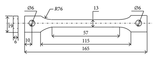
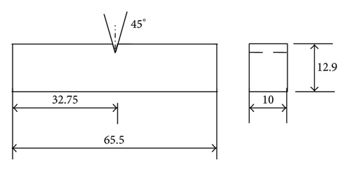
The experimental building material adopted is CIBATOOL 5530 epoxy resin. The experimental building models are categorized into three specimens, namely, the tensile test (Figure 1), flexural test (Figure 2), and impact test (Figure 3), and are characterized using ASTM D638-01 [16], ASTM D790-03 [17], and ASTM D256-04 [18] specifications, respectively. The STL format is generated by CATIA V5 R16 and sent to the 3D system SLA 5000 rapid prototyping machine. The various conditions in preprocessing steps such as STL verification, deposition layer thickness, orientation, building interior structure form, supporting method, and building deposition direction are incorporated by means of 3D light year software [19] provided by 3D system of Valencia, USA, followed by the layer slicing process to generate the building path with ACES build style. Building quality characteristics or attributes include the-larger-the-better (LB) for the strength of the SLA prototypes.

2.1. Experimental Apparatus
The major experimental apparatus adopted includes 3D system SLA5000 rapid prototyping machine produced by the Valencia, USA, where it uses CIBATOOL 5530 epoxy resin to build geometrical shape of the work piece by photopolymerization process. Similarly, the tensile and flexural tests were conducted using Instron Universal Testing Machine, UK, Model 5582. The impact test was conducted using impact tester, Aditya Instruments, Bangalore, Model IT-30.
2.2. Taguchi Quality Engineering
The orthogonal array is employed for the Taguchi method as the experimental analysis basis. The experimental factors and their corresponding levels are identified. Then the experimental results are manipulated and validated by analysis of variance (ANOVA), in order to determine each factor effect versus the response variable strength of the SLA prototypes. The experimental procedures are given as follows: identification of SLA process parameter that influences the response variable and determining the various levels of the factors. Based on the factors and their levels, the degree of freedom is calculated and the suitable orthogonal array is selected and the experiment proceeds according to the variable factor layout of the orthogonal array. The experimental results are obtained and the signal to noise ratio (S/N ratio), the ANOVA, and the corresponding contribution are computed, obtaining the empirical relationship for the response variable under different parameter settings.
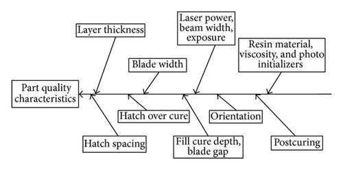
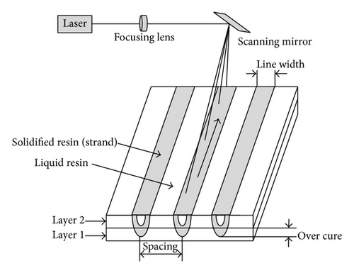
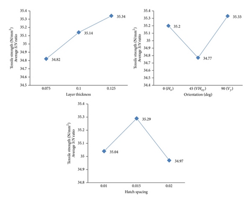
Figure 4 shows the probable parameters (causes) that influence the part quality characteristics (effects) in the SLA process. Figure 5 represents the various process parameters of SLA process, and among these the layer thickness (Lt) is the thickness where the model is sliced in the Z direction, orientation (O) is the position in which the prototype is built, and hatch spacing (Hs) is the narrow region solidified by the laser scanning. If the strand is located at the top or bottom surface of part, spacing is called fill spacing otherwise hatch spacing, which are the parameters that influence the strength of the SLA parts [23]. Table 1 provides the three levels of the process parameters for the experimentation.
| Symbol | Control parameters | Level 1 | Level 2 | Level 3 |
|---|---|---|---|---|
| A | Layer thickness (Lt) | 0.075 | 0.1 | 0.125 |
| B | Orientation (O) | 0° (Hx) | 45° (VHxy) | 90° (Vy) |
| C | Hatch spacing (Hs) | 0.01 | 0.015 | 0.02 |
The total number of experiments in full factorial design for “m” parameters in each set of “L” levels is Lm and it increases exponentially with L & m. Taguchi suggested the use of orthogonal array which will be used for conducting the fractional factorial experiments [24]. The Taguchi orthogonal array adopted in the research experiment is L9 for three-factor three-level settings as shown in Table 2.
| Experimental run (j) | Levels | ||
|---|---|---|---|
| A | B | C | |
| Layer thickness (Lt)—mm | Orientation (O)—° | Hatch spacing (Hs)—mm | |
| 1 | 1 | 1 | 1 |
| 2 | 1 | 2 | 2 |
| 3 | 1 | 3 | 3 |
| 4 | 2 | 1 | 2 |
| 5 | 2 | 2 | 3 |
| 6 | 2 | 3 | 1 |
| 7 | 3 | 1 | 3 |
| 8 | 3 | 2 | 1 |
| 9 | 3 | 3 | 2 |
3. Experimentation
3.1. Experimental Analysis for Tensile Strength (Ts)
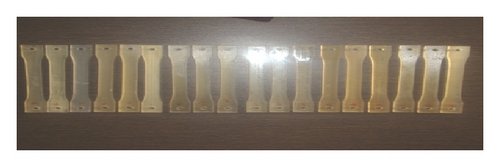
The nine tensile specimens as per the ASTM standards (ASTM D638-01) were built for L9 orthogonal array setting using epoxy resin CIBATOOL SL5530 in SL5000 machine of three replications each. The dimensional details of the test specimen are given in Figure 1 [16] and the SLA prototypes are as shown in Figure 6. The tensile strength is calculated using the ratio of ultimate load to cross sectional area. The experimental results are given in Table 3.
| j | 1 | 2 | 3 | 4 | 5 | 6 | 7 | 8 | 9 |
|---|---|---|---|---|---|---|---|---|---|
| Tsj (N/mm2) | 55.46 | 54.57 | 55.07 | 58.46 | 54.51 | 58.59 | 58.62 | 55.34 | 61.73 |
3.1.1. Prediction of Optimal Levels of Process Parameters
-
layer thickness: 0.125 mm (level 3, S/N ratio: 35.34),
-
orientation: 90° Vy (level 3, S/N ratio: 35.33),
-
hatch spacing: 0.015 (level 2, S/N ratio: 35.29).
| Parameters | Level | Expm run | Tsj (N/mm2) | nj | navg |
|---|---|---|---|---|---|
| Layer thickness | 1 (0.075) | 1 | 55.46 | 34.89 | 34.82 |
| 2 | 54.57 | 34.74 | |||
| 3 | 55.07 | 34.82 | |||
| 2 (0.1) | 4 | 58.46 | 35.34 | 35.14 | |
| 5 | 54.51 | 34.73 | |||
| 6 | 58.59 | 35.36 | |||
| 3 (0.125) | 7 | 58.62 | 35.36 | 35.34 | |
| 8 | 55.34 | 34.86 | |||
| 9 | 61.73 | 35.81 | |||
| Orientation | 1 (0°) | 1 | 55.56 | 34.89 | 35.2 |
| 4 | 58.46 | 35.34 | |||
| 7 | 58.62 | 35.36 | |||
| 2 (45°) | 2 | 54.57 | 34.74 | 34.77 | |
| 5 | 54.51 | 34.73 | |||
| 8 | 55.34 | 34.86 | |||
| 3 (90°) | 3 | 55.07 | 34.82 | 35.33 | |
| 6 | 58.59 | 35.36 | |||
| 9 | 61.73 | 35.81 | |||
| Hatch spacing | 1 (0.01) | 1 | 55.56 | 34.89 | 35.04 |
| 6 | 58.59 | 35.36 | |||
| 8 | 55.34 | 34.86 | |||
| 2 (0.015) | 2 | 54.57 | 34.74 | 35.29 | |
| 4 | 58.46 | 35.34 | |||
| 9 | 61.73 | 35.81 | |||
| 3 (0.02) | 3 | 55.07 | 34.82 | 34.97 | |
| 5 | 54.51 | 34.73 | |||
| 7 | 58.62 | 35.36 | |||
3.1.2. Identification of Significance and Percentage of Contribution of Process Parameters
The process parameters (Lt, O, and Hs) which have more influence on the response variable are identified through the percentage of contribution of each parameter. The parameter which has more percentage of contribution is the significant parameter to the response variable [25–28]. They have mentioned that ANOVA is widely used for determining the significance of the independent variables in influencing the dependent variables and also in determination of percentage of contribution of these dependent variables to the response variable.
Table 5 shows the percentage of contribution of the parameters to the response variable with the ANOVA parameters. Hence, from the ANOVA table the significance of each parameter is identified.
| Parameter “i” | Sum of squares | Degree of freedom | Mean sum of squares | F statistics | F tabulated | % of contribution |
|---|---|---|---|---|---|---|
| F(0.1,2,2) | ||||||
| Lt | 18.57 | 2 | 9.285 | 9.622* | 36.93 | |
| O | 21.72 | 2 | 10.86 | 11.25* | 9 | 43.19 |
| Hs | 8.06 | 2 | 4.03 | 4.176 | 16.03 | |
| Error | 1.93 | 2 | 0.965 | 3.83 | ||
| Total | 50.28 | 8 | 25.14 | |||
- *Significance at 90% confidence level (F statistics > F tabulated).
3.2. Experimental Analysis for Flexural Strength (Fs)
| j exp., run | 1 | 2 | 3 | 4 | 5 | 6 | 7 | 8 | 9 |
|---|---|---|---|---|---|---|---|---|---|
| FSj (N/mm2) | 116.67 | 113.92 | 114.08 | 115.7 | 110.0 | 115.6 | 115.8 | 114.8 | 118.7 |
| Parameters | Level | Expn run | Fsj (N/mm2) | nj | navg |
|---|---|---|---|---|---|
| Layer thickness | 1 (0.075) | 1 | 116.67 | 41.33 | 41.2 |
| 2 | 113.92 | 41.13 | |||
| 3 | 114.08 | 41.14 | |||
| 2 (0.1) | 4 | 115.7 | 41.26 | 41.11 | |
| 5 | 110.0 | 40.82 | |||
| 6 | 115.6 | 41.25 | |||
| 3 (0.125) | 7 | 115.8 | 41.27 | 41.32 | |
| 8 | 114.8 | 41.20 | |||
| 9 | 118.7 | 41.49 | |||
| Orientation | 1 (0°) | 1 | 116.67 | 41.33 | 41.28 |
| 4 | 115.7 | 41.26 | |||
| 7 | 115.8 | 41.27 | |||
| 2 (45°) | 2 | 113.92 | 41.13 | 41.05 | |
| 5 | 110.0 | 40.82 | |||
| 8 | 114.8 | 41.20 | |||
| 3 (90°) | 3 | 114.08 | 41.14 | 41.30 | |
| 6 | 115.6 | 41.25 | |||
| 9 | 118.7 | 41.49 | |||
| Hatch spacing | 1 (0.01) | 1 | 116.67 | 41.33 | 41.26 |
| 6 | 115.6 | 41.25 | |||
| 8 | 114.8 | 41.20 | |||
| 2 (0.015) | 2 | 113.92 | 41.13 | 41.29 | |
| 4 | 115.7 | 41.26 | |||
| 9 | 118.7 | 41.49 | |||
| 3 (0.02) | 3 | 114.08 | 41.14 | 41.08 | |
| 5 | 110.0 | 40.82 | |||
| 7 | 115.8 | 41.27 | |||

-
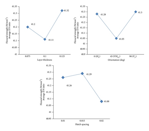
layer thickness: 0.125 mm (level 3, S/N ratio: 41.32),
-
orientation: 90° Vy (level 3, S/N ratio: 41.3),
-
hatch spacing: 0.015 (level 2, S/N ratio: 41.29).
| Parameter “i” | Sum of squares | Degree of freedom | Mean sum of squares | F statistics | F tabulated | % of contribution |
|---|---|---|---|---|---|---|
| F(0.01,2,2) | ||||||
| Lt | 10.75 | 2 | 5.375 | 82.69 | 23.88 | |
| O | 20.3 | 2 | 10.15 | 156.15* | 99 | 45.09 |
| Hs | 13.84 | 2 | 6.92 | 106.45* | 30.75 | |
| Error | 0.13 | 2 | 0.065 | 0.28 | ||
| Total | 45.02 | 8 | 22.507 | |||
- *Significance at 99% confidence level (F statistics > F tabulated).
3.3. Experimental Analysis for Impact Strength
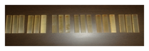
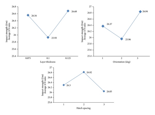
The analysis carried out for the impact strength is identical to the one in Section 3.1. The nine impact test specimens as per the ASTM standards (ASTM D256-04) are built for L9 orthogonal array setting using epoxy resin CIBATOOL SL5530 in SL5000 machine of three replications each. The dimensional details of the test specimen are given in Figure 3 [18] and the SLA prototypes are shown in Figure 10. In Izod test method, the specimen is placed vertically and is broken by a single swing of the pendulum weight with a contact point at a fixed distance from the centerline of the notch. The impact strength is obtained through the ratio of energy absorbed by the specimen during the break and the width of the specimen using Izod impact tests. The experimental results of impact strength are tabulated in Table 9. Table 10 shows the S/N ratio for each of the levels in each factor and Figure 11 shows the variation of S/N ratio for all the controllable factors.
| j exp., run | 1 | 2 | 3 | 4 | 5 | 6 | 7 | 8 | 9 |
|---|---|---|---|---|---|---|---|---|---|
| ISj (J/m) | 20.8 | 22 | 21.1 | 20.3 | 17.9 | 21.3 | 21.4 | 19.9 | 23.6 |
| Parameters | Level | Experimental run | Isj (J/m) | nj | navg |
|---|---|---|---|---|---|
| Layer thickness | 1 (0.075) | 1 | 20.8 | 26.36 | 26.56 |
| 2 | 22 | 26.85 | |||
| 3 | 21.1 | 26.48 | |||
| 2 (0.1) | 4 | 20.3 | 26.15 | 25.93 | |
| 5 | 17.9 | 25.06 | |||
| 6 | 21.3 | 26.57 | |||
| 3 (0.125) | 7 | 21.4 | 26.61 | 26.68 | |
| 8 | 19.9 | 25.97 | |||
| 9 | 23.6 | 27.46 | |||
| Orientation | 1 (0°) | 1 | 20.8 | 26.36 | 26.37 |
| 4 | 20.3 | 26.15 | |||
| 7 | 21.4 | 26.61 | |||
| 2 (45°) | 2 | 22 | 26.85 | 25.96 | |
| 5 | 17.9 | 25.06 | |||
| 8 | 19.9 | 25.97 | |||
| 3 (90°) | 3 | 21.1 | 26.48 | 26.84 | |
| 6 | 21.3 | 26.57 | |||
| 9 | 23.6 | 27.46 | |||
| Hatch spacing | 1 (0.01) | 1 | 20.8 | 26.36 | 26.3 |
| 6 | 21.3 | 26.57 | |||
| 8 | 19.9 | 25.97 | |||
| 2 (0.015) | 2 | 22 | 26.85 | 26.82 | |
| 4 | 20.3 | 26.15 | |||
| 9 | 23.6 | 27.46 | |||
| 3 (0.02) | 3 | 21.1 | 26.48 | 26.05 | |
| 5 | 17.9 | 25.06 | |||
| 7 | 21.4 | 26.61 | |||
-
layer thickness: 0.125 mm (level 3, S/N ratio: 26.68),
-
orientation: 90° Vy (level 3, S/N ratio: 26.84),
-
hatch spacing: 0.015 (level 2, S/N ratio: 26.82).
| Parameter “i” | Sum of squares | Degree of freedom | Mean sum of squares | F statistics | F tabulated | % of contribution |
|---|---|---|---|---|---|---|
| F(0.01,2,2) | ||||||
| Lt | 5.5 | 2 | 2.75 | 2.69 | 28.47 | |
| O | 6.44 | 2 | 3.22 | 3.16* | 3 | 33.33 |
| Hs | 5.34 | 2 | 2.67 | 2.617 | 27.64 | |
| Error | 2.04 | 2 | 1.02 | 10.55 | ||
| Total | 19.32 | 8 | 9.66 | |||
- *Significance at 75% confidence level (F statistics > F tabulated).
4. Establishment of Process Model (Regression Equation)
4.1. Empirical Relation for Tensile Strength versus Process Parameters
| Levels | Linear | Nonlinear |
|---|---|---|
| Lower | −1 | 1 |
| Medium | 0 | −2 |
| Higher | 1 | 1 |
4.2. Empirical Relation for Flexural Strength versus Process Parameters
4.3. Empirical Relation for Impact Strength versus Process Parameters
5. Conclusions
- (i)
Parameters Lt, O, and Hs influence much on part strength of SLA prototypes.
- (ii)
The optimal level combination of the process parameters is as follows:
-
layer thickness: 0.125 mm (level 3),
-
orientation: 90°Vy (level 3),
-
hatch spacing: 0.015 (level 2),
-
-
for tensile, flexural, and impact strength of the SLA prototypes.
- (iii)
Among the three process parameters, the Lt and O are major contributing parameters for the tensile strength, O and Hs are major contributing parameters for the flexural strength, and O has more significance among the parameters for the impact strength.
- (iv)
The empirical relationship (process model) between the part strength characteristics and the influencing parameters has been established for stereolithography process, which can predict the strength of the SLA prototypes by prior knowledge of part strength before building the prototypes.
- (v)
The layer thickness plays an important role since the SLA process has an inbuilt specific property of building the prototypes with layer by layer method.
Conflict of Interests
The authors declare that there is no conflict of interests regarding the publication of this paper.
Acknowledgments
The authors would like to thank the management of Reva Institute of Technology and Management, Bangalore, and the Director of the Gas Turbine Research Establishment, Bangalore, and Sriram Industries, Bangalore, for their immense help to carry out this work.


