Performance of Various Metaheuristic Techniques for Economic Dispatch Problem with Valve Point Loading Effects and Multiple Fueling Options
Abstract
The paper presents the metaheuristic approaches based on pattern search and simulated annealing hybridized with sequential quadratic programming, a powerful nonlinear adaptive technique for estimation of the finest combination of generated power in a given system at lowest operating cost while sustaining the operating condition of system efficiently. The fuel cost is minimized by satisfying the nonlinear operating conditions of thermal units mainly based on generation capacity constraints, generator ramp limit, power balance constraints, and valve point loading effect and by keeping in view the prohibited operating zones, respectively. About the optimization, a comparative study is made for pattern search (PS) and simulated annealing (SA), as a viable global search technique and sequential quadratic programming, an efficient local optimizer and their hybrid versions. The applicability, stability, and reliability of the designed approaches are validated through comprehensive statistical analysis based on Monte Carlo simulations.
1. Introduction
The performance and designing of electric power system serve two purposes; one is to maintain the economy and the other is to include reliability of the system [1]. Economic dispatch problem (EDP) is one of the significant optimization problems in industrial independent power system and acquires increasing importance as the operating cost and electric energy demand is increasing globally around the planet [2, 3]. The procedure involves dividing the power demand of generating system for online thermal units in such manner that their operating cost is optimal while satisfying the power demand to the user and constraint adequately [3, 4]. Since the operating cost of generating unit is inflated an optimal EDP can lead to prominent cost saving with reducing the atmospheric emission of thermal power plant [4]. In the energy crises age, a number of engineers and scientists are taking interest in the optimized solution of this industrial problem [5] by keeping in view the constraints like generator ramp limit, power balance, and valve point loading effect (VPLE) and prohibited operating zones [6, 7]. However the facts of EDP with multiple fueling option (MFO) and MFO combined with VPLE conditions is not well addressed simultaneously, which are the motivations for taking this study with metaheuristic computing approach.
Traditional numerical models and programming strategies have been developed, like lambda iteration method, quadratic programming, Lagrangian relaxation algorithm, base point participation factor, gradient method linear programming, reduced gradient method, piecewise linear cost function, Newton method, and dynamic programming [8, 9], but all these EDP tools are flexible and applicable if the function between operating cost and fuel or heat are piecewise linear and increasing categorically [10]. Modern approaches use artificial neural network models which show dominance on classical techniques [11], while its parameters can overwrite during the learning in complex constraints based EDP problems. In order to overcome this issue the metaheuristic approaches based on tabu search, Hopfield, hill climbing, evolutionary computation, swarm intelligence, and ant/bee colony optimizations can outperform [12, 13].
In the recent development on optimization technique for EDP problems, multiperiod hydrothermal economic dispatch is employed with an efficient local search based on interior point method [14] that has an issue of getting stuck in the local minima. The solution of unit commitment problem is addressed by a hybrid scheme based on modified subgradient method and simulating annealing algorithm [15]; this combination of derivative based and derivative free method is good but with the constraints of high computational budget involved in its computations. The predictor corrector primal dual interior point algorithm is well presented in [16] in terms of computational cost for solving EDP problem; however the mean level of accuracy is not well matured. Parametric approach involved in parameter setting free harmony search and parallel adaptive algorithm schemes are established for economic dispatch and environmental power dispatch problems, respectively [17, 18]. With all this recent development, this paper presents the comprehensive analysis in terms of minimum fuel cost, level of accuracy in the optimizer, statistical analysis on computational budget needed, and convergence rate as well, on complex dynamical version of EDP problem involving MFO and VPLE conditions. The presented work is compared with [19–21], in which EDP problem has been exploited by evolutionary strategy, standard particle swarm optimization (PSO), Gaussian PSO, and chaotic PSO, respectively.
The remaining of this paper is organized as follows: Section 2 describes the formulation of an EDP along with the constraints. The proposed methodology along with the procedural hybrid step is revealed in Section 3. Section 4 discusses the computational procedure and analyzes the results when applied to the scenarios of EDPs with 13, 15, and 20 thermal units. The last section of the paper outlines the conclusions drawn from the simulation and results along with some directions for the future research.
2. Economic Dispatch Problem Formulation
The objective of EDP is to find the finest combination of generated power in a given system at lowest operating cost while sustaining the operating condition of system efficiently by satisfying the nonlinear operating conditions formulated as follow.
2.1. Fuel Cost Minimization
2.2. Inequality Constraint
2.2.1. Generation Capacity Constraint
2.2.2. Generator Ramp Limit
2.2.3. Power Balance Constraint
2.3. Valve-Point Loading Effect (VPLE)
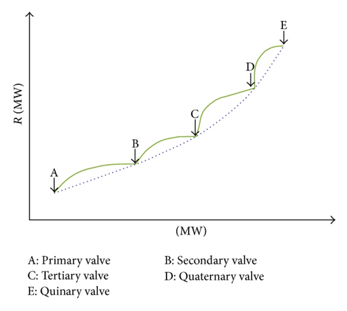
For a power plant having NG committed units have multivalve opening sequence to meet the fluctuating loads demand. VPLE introduce ripples in the input-output characteristics of generating units resultantly making the heat curve rate nonconvex with increase in unit loading. Heat rate curve decreases between the opening points of two valves as shown in Figure 1 [23].
2.4. Prohibited Operating Zones
2.5. EDP with Multiple-Fueling Option (MFO)
2.6. EDP Considering Both VPLE and MFO
3. Proposed Methodology
The brief introduction of optimizers used for optimization of EDP is narrated along with the necessary detail of hybrid algorithm in the form of procedural steps.
3.1. Simulated Annealing
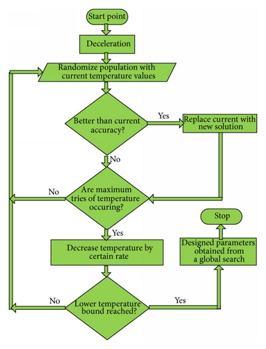
Simulated annealing is heuristic as well as probabilistic method proposed by Scott Kirkpatrick, C. Daniel Gelatt, and Mario P. Vecchi in 1983 for localizing better approximation to find global minimum of given cost function that may be surrounded with several local minima in a large search space [24]. SA is more efficient as compared with hill climbing and is a good choice for engineers and researchers to handle complex nonlinear systems especially problems like EDP due to its coding leniency to get guarantee finest optimal solutions. The method works on the principle of randomly initializing of finite solution space of specific size N on the basis of scattered neighborhood points that mimic from the principle of thermal annealing of solids [25]. The decreasing of temperature at a specific rate in each iteration resembles the optimization of the merit function of EDP subject to varying the heat values as adaptive parameters of a specific problem. The candidate solution is updated based on the values of the fitness in terms of mean square error of the previous possible solution along with the index term; on this basis the iterative process matures towards the region of convergence of the fitness function. SA belongs to the family of global search techniques so it has various start points in the start of the algorithm to avoid local minimum. Usually the number of iterations of SA is very large while the computational budget is quite reasonable for most of the test bench problem. Although, it has been applied in various areas of engineering, some key applications are found in crystallographic refinement, neural computing [26], optimal reconfiguration of distribution networks, wireless communication, phase balancing, van der pol oscillators involved in mechanical engineering [27], and combinatorial optimization problem [28]. The generic flow diagram used for the simulated annealing algorithm is provided in Figure 2.
3.2. Pattern Search
Pattern search (PS) is numerical optimization method proposed by Hooke and Jeeves [29] for statistical problems and main advantages of PS are that it is efficient and computational structure is simple to understand and also it does not required gradient of cost function so it can be used in functions that are not constant or not differentiable and method is also known as direct-search, derivative-free approaches. Pattern search algorithm searches for a sequence of points to reach an optimal solution by initializing a set of points called mesh. The mesh formation procedure is involved by adding a pattern vector to the initial point and if PS acquires a point in mesh that refines the objective function then the new point becomes the current point at the next step of the algorithm [30].
Usually the practical nonlinear optimization problem of power system lies outside the reach of the standard optimization techniques. The practical EDP problems can be optimized by PS which is computationally efficient and easy to implement as compared to other heuristic techniques [31]. PS initializes by computing sequence of point that may or may not be reached optimally and established a set point called mesh around these given points. This current point could be a starting point provided by user or extracted from previous step of algorithm. Current points are then added to a pattern vector which is scalar multiple of a set of vectors for mesh formation. If an objective function is improved by point in mesh then the new point becomes the current point at the next iteration [32].
Pattern search is efficient optimization techniques applied in areas of parallel computing, pattern character recognition, graphic user interference thermal control systems, nonlinear and optimal control theory [33], and so forth.
3.3. Sequential Quadratic Programming
The SQP algorithm is one of the nonlinear programming techniques used extensively by the research community for constraints optimization problems. The strength of the scheme is well-established in terms of efficiency, accuracy, and percentage of successful solutions over a large number of test problems. Thum and Schilling [34] have provided excellently a brief introduction and description of SQP algorithms. As the physics of SQP is based on local search techniques so it is more probable to get stuck in the local minimum so some of the iterations during Monte Carlo simulation can show divergence or least accuracy. However the rate of convergence and level of accuracy for successful runs is dramatically high for SQP algorithms. The detailed history, mathematical formulation, importance, and application related with SQP methods can be seen in [35, 36]. The SQP methods have been applied on broad disciplines of engineering and applied science from the day of their birth to today; for instance, few recently published articles addressing SQP technique are referred to for interested readers in [37, 38].
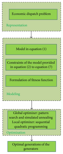
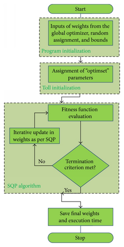
Now the intention is to formulate the overall procedure and the optimization of the unknown designed parameters of the units generation along with the fuel cost; the process of the proposed scheme is provided in Figure 3. The modeling is performed based on relations provided in (1) and relations of constraints, respectively. The optimization is performed using global versions of simulated annealing and pattern search hybrid with sequential quadratic programming, an efficient local search technique. In Figure 3(b) the designed parameters obtained from global optimizer are provided as a start point to SQP for further tuning of the design. The algorithm used for the optimization of EDP in the form of the logical steps based on hybrid computational technique is as follows.
Step 1 (population generation). A random and well scattered population of size M is generated with agents of length exactly equal to the number of power generating units N.
In general the ith agent of the candidate solution is represented by ci = [ci1, ci2, …, ciN], , j = 1,2, 3, …, M, where Lb and Ub are the lower and upper possible limits to generate power.
Step 2 (initialization). Initialize and assign the general and specific values for parameter setting involved in pattern search and simulated annealing algorithm as provided in Table 1.
| PS | SA | ||
|---|---|---|---|
| Parameters | Settings | Parameters | Setting |
| Poll method | MADS positive basis 2N | Start point size | 15 |
| Poll order | Random | Population size | 300 |
| Mesh size | (1, 15) | Annealing function | Boltzmann |
| Expansion factor | 2.5 | Reannealing interval | 150 |
| Contraction factor | 0.7 | Temperature update | Exponential |
| Penalty factor | 150 | Initial temperature | 100 |
| Initial range | [0-1] | Bound | Problem specific |
| Maximum function Evaluations | 30000 | Maximum function evaluation | 45000 |
| Maximum iterations | 1500 | Maximum iterations | 1500 |
| Others | Default | Others | Default |
Step 3 (fitness evaluation). Find the fitness of each agent using the fitness evaluation function ξ as given below in the form of mean square error (MSE):
Step 4 (termination criteria). The algorithm is terminated on the basis of the following criteria.
Step 5 (reproduction). New population is generated using the operations evolved in PS and SA as per the setting given in Table 1 and then go to Step 3.
Step 6 (refinement via SQP method). One of the best results obtained by PS and SA is provided to SP as a start point for further refinement, and the parameter setting and values used for SQP algorithm are provided in Table 2.
| Sequential quadratic programming | |
|---|---|
| Parameters | Settings |
| Start point | Final weights of PS or SA |
| Bounds | Specific lower and upper limit of generators |
| X-tolerance | 10−12 |
| Function tolerance | 10−12 |
| Hessian | BFGS |
| Scaling | Objective and constraints |
| Maximum iterations | 1000 |
| Maximum function evaluations | 1500 |
| Others | Default |
Step 7 (storage). Store the global best of this cycle and repeat the procedure from Steps 3 to 7, to get sufficient numbers of independent runs to have sufficient data for performing analysis.
Step 8 (statistical analysis). The statistical analysis is made on the basis of four fundamental performance modes like best, worst, mean, and standard deviation and skewness.
4. Simulation and Results
In this section, a scenario based simulation is performed based on three case studies composed of thirteen, fifteen, and twenty generating units, respectively, for EDP problem in which the objective functions were ramp rate limit, prohibited operating zones in the power system operation; MFO and VPLE and transmission losses are also employed to demonstrate efficiency of proposed schemes using MATLAB built in subroutines of the optimizers like PS, SA, SQP, PS-SQP, and SA-SQP, respectively, whose parameters setting and values are provided in Tables 1 and 2. The reference data sheet for thirteen thermal units [37] with load demand of 3080 MW is provided in Appendix A. The data set used for fifteen thermal units [19–21] along with generating unit capacity, coefficients, ramp rate limits, and prohibited zones is provided in Appendix B while the load demand expected to be determined is 2630 MW. However, the data sheet for twenty thermal units of generating unit capacity and coefficients [38] are provided in Appendix C, where system supplies a total load demand of 2500 MW.
One of the best designed parameters is in fact the power generating values of generators and is presented in Figure 4 at semilog scale in order to widen the small effects in the power values. The lowest cost of the power generation can be obtained by taking the generating values from the hybrid schemes based on PS-SQP and SA-SQP, respectively, from Figures 4(a), 4(b), and 4(c) in fitness evaluation function provided in (10) along with the subsequent relations given in (1) and expressions of EDP constraints. The x-axis in Figure 4 defines the number of thermal units taken in the study and y-axis demonstrates the solvers PS, SA, SQP, PS-SQP, and SA-SQP, respectively, while z-axis provides the optimized values of the power for thermal units.
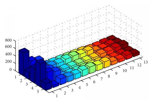
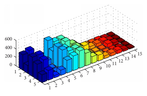
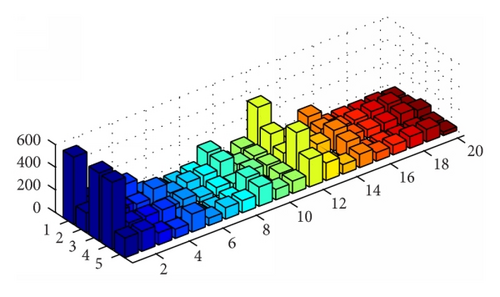
The optimized final values along with computational time for PS, SA, SQP, PS-SQP, and SA-SQP are provided in Table 3. The time analysis carried out for this paper is on Intel(R) Core (TM) i5-3210M CPU @ 2.50 GHz, 2.5 GHz, 4.0 GB of RAM, and running with MATLAB version 2012a. It is quite evident from the table that level of accuracy is dominated in case of hybrid schemes as compared to global search and local search techniques separately. However the computational budget of hybrid approach is a little bit more as compared to other presented schemes but this effect can be over shed due to the high accuracy attained by hybrid schemes. The local search scheme seems to be outperformed in terms of both accuracy and computational cost; however one cannot rely on one of these best values of SQP as the local search techniques are more probable to get stuck in the local optima due to bad initial guess. Another observation is that as the number of generating units increases the level of accuracy reduces while computational time increases due to increase in the EDP complexity.
| Scenarios | PS | SA | SQP | PS-SQP | SA-SQP | |||||
|---|---|---|---|---|---|---|---|---|---|---|
| Fval | τ | Fval | τ | Fval | τ | Fval | τ | Fval | τ | |
| Case 1 | 2.01E − 13 | 0.29975 | 1.25E − 15 | 26.9359 | 5.24E − 19 | 0.09749 | 8.95E − 21 | 0.22732 | 8.40E − 19 | 0.05562 |
| Case 2 | 1.84E − 11 | 1.68357 | 1.20E − 16 | 29.8246 | 1.22E − 11 | 2.98696 | 2.90E − 13 | 1.10707 | 1.00E − 19 | 0.24536 |
| Case 3 | 2.01E − 13 | 0.29975 | 1.25E − 15 | 26.9359 | 5.24E − 19 | 0.09749 | 8.95E − 21 | 0.22732 | 8.40E − 19 | 0.05562 |
The reliability of the stochastic algorithms is being tested by a comprehensive statistical analysis in terms of minimum of cost (Mincost), maximum value of cost (Maxcost), mean cost value (Meancost), and standard deviation of the cost (STDcost). The analysis is not only performed on cost value but also performed on computational time needed for the optimization in term of mean CPU (MeanCPU) time. The results of the Monte Carlo simulations for stochastic solvers are narrated in Tables 4 and 5 for fifteen and twenty units, respectively, while for thirteen units the same analysis is provided in Appendix D.
| Method | Mincost | Meancost | STDcost | Maxcost | MeanCPU time |
|---|---|---|---|---|---|
| Evolutionary strategy [19] | 32568.54 | 32620.00 | — | 32710.00 | 0.48 |
| PSO [20] | 33858.00 | 33039.00 | — | 3331.000 | 26.59 |
| Genetic algorithm [20] | 33113.00 | 33228.00 | — | 3337.000 | 49.31 |
| Gaussian PSO [21] | 32508.12 | 35122.79 | 1918.62 | 38044.42 | 0.69 |
| Chaotic PSO [21] | 32775.68 | 35340.70 | 1942.84 | 38104.54 | 0.59 |
| Proposed | |||||
| PS | 33154.10 | 34908.12 | 1712.34 | 36.001.14 | 0.640587 |
| SA | 33124.24 | 35012.54 | 1612.35 | 36312.12 | 22.78067 |
| SQP | 32567.45 | 33467.14 | 1712.12 | 35123.90 | 0.418991 |
| PS-SQP | 32005.00 | 32145.23 | 1735.12 | 32568.28 | 1.059578 |
| SA-SQP | 32000.14 | 32112.12 | 1659.38 | 32412.02 | 23.199661 |
| Method | Mincost | Meancost | STDcost | Maxcost | MeanCPU time (s) |
|---|---|---|---|---|---|
| Lambda iteration method [38] | 62456.6391 | — | — | — | 0.033 |
| Hopfield neural networks [38] | 62456.6341 | — | — | — | 0.006 |
| Gaussian PSO [21] | 60526.15 | 61123.36 | 330.89 | 62757.19 | 0.50 |
| Chaotic PSO [21] | 60803.51 | 61223.95 | 507.56 | 62982.19 | 0.37 |
| Proposed | |||||
| PS | 59829.15 | 61256.21 | 1342.56 | 63125.56 | 1.054175 |
| SA | 59803.45 | 61002.34 | 1423.89 | 62340.16 | 32.31666 |
| SQP | 57231.43 | 59012.45 | 1712.35 | 60123.23 | 0.294808 |
| PS-SQP | 58123.98 | 58563.65 | 976.140 | 58901.26 | 1.348983 |
| SA-SQP | 57120.21 | 58011.78 | 658.341 | 58764.38 | 33.643791 |
It is quite evident from Tables 4 and 5 that the results of the proposed schemes are in good agreement in terms of reliability, effectiveness, economical cost, and computational budget required in terms of time complexity; however the hybrid approaches PS-SQP and SA-SQP show more supremacy than that of PS, SA, and SQP. The computational budget of hybrid schemes seems to computationally heavy of order of just few seconds; however this aspect seems to be minimal at the cost of level of accuracy achieved.
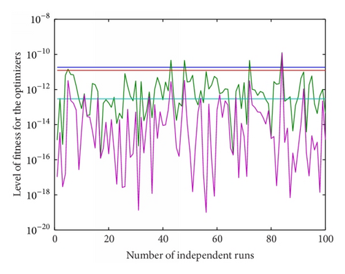
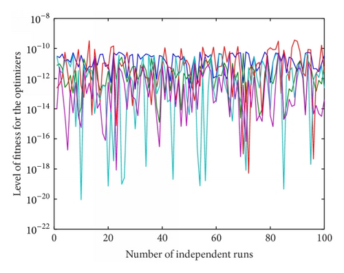
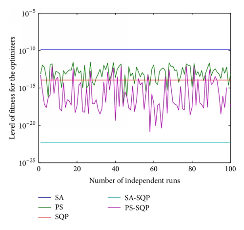
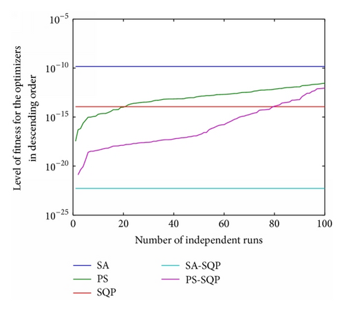
As the proposed scheme is based on heuristic computation one of the best results cannot define the effectiveness and reliability of the schemes; therefore in order to see the effectiveness of given stochastic methods the results are obtained for hundred independent runs rather on a single successful run. The fitness given in (10) obtained on all independent iterations is plotted in Figure 5 for three variations of generating units.
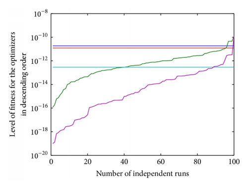
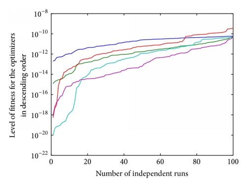
The percentage of convergence is also calculated by fixing a certain level of the threshold (ξ ≤ 10−10) in the level of fitness obtained by all proposed algorithms and the results are plotted in Figure 6 at four hundred independent runs of the given algorithms. It is observed from Figure 6(a) that all the optimizers provide 100% convergence for EDP with thirteen thermal units while for the case of fifteen units the convergence for SA is 97% and 100% for rest of the algorithms. Scenario three that is relatively stiff does not show convergence for PS on a threshold of (ξ ≤ 10−10), while the other optimizers like SA, SQP, PS-SQP, and SA-SQP are 100% convergent as evident from Figure 6(c).
5. Conclusions
On the basis of the results obtained by various optimizers in the last sections, the following conclusion can be drawn.
The proposed scheme based on SA-SQP and PS-SQP hybrid algorithms can provide reliable, effective, and well optimized cost of EDP for the scenarios of thirteen, fifteen, and twenty thermal units for a demand of 3080 M, 2630 MW, and 2500 MW, respectively.
The comparative study between the solvers is carried out in terms of absolute cost, computational complexity, and fitness value achieved by the PS, SA, SQP, PS-SP, and SA-SP algorithms. The hybrid algorithms are found to be better than that of global and local search techniques applied independently for all variants of ESPs.
The results of statistical analysis determined for 100 independent runs of the design approaches show that the values in terms of mean, standard deviation, and minimum of the total cost error associated with PS-SQP and SA-SQP are considerably more dominated than SA, PS, and SQP techniques. The value of the mean execution time for finding the optimal weight with proposed schemes shows that the hybrid approaches take relatively more time than the other three techniques but this exception can be overshadow due to its utmost accuracy and consistently convergent performance.
At a fitness threshold of ε ≤ 10−10, the algorithms based on hybrid schemes on average provide 100% convergence while the convergences of SA and PS are observed to be in a good range of acceptance, although in same situations PS remains consistent due to the same creation of mesh in the polling and searching domain.
The main advantages of given schemes lie in their ease in implementation, simplicity in the concept, minimal computational complexity, less hardware implementation burden, and suitability for real-time applications. In future, one may look for biological inspired computational method to analyze synthesis and optimize the other dynamical constraint based EDPs problems.
Conflict of Interests
The authors declare that there is no conflict of interests regarding the publication of this paper.
Appendices
A. Generating Units Capacity and Coefficients (13 Units)
See Table 6.
| Units | (MW) | (MW) | a ($/MW2) | b ($/MW2) | c ($/MW2) |
|---|---|---|---|---|---|
| 1 | 0 | 680 | 0.00028 | 8.10 | 550 |
| 2 | 0 | 360 | 0.00056 | 8.10 | 309 |
| 3 | 0 | 360 | 0.00056 | 8.10 | 307 |
| 4 | 60 | 180 | 0.00028 | 7.74 | 240 |
| 5 | 60 | 180 | 0.00324 | 7.74 | 240 |
| 6 | 60 | 180 | 0.00324 | 7.74 | 240 |
| 7 | 60 | 180 | 0.00324 | 7.74 | 240 |
| 8 | 60 | 180 | 0.00324 | 7.74 | 240 |
| 9 | 60 | 180 | 0.00324 | 7.74 | 240 |
| 10 | 40 | 120 | 0.00284 | 8.60 | 126 |
| 11 | 40 | 120 | 0.00284 | 8.60 | 126 |
| 12 | 55 | 120 | 0.00284 | 8.60 | 126 |
| 13 | 55 | 120 | 0.00284 | 8.60 | 126 |
B. (a) Generating Units Capacity and Coefficients (15 Units) (b) Ramp-Rate Limits and Prohibited Zones (15 Units)
See Table 7.
| Units | (MW) | (MW) | a ($/MW2) | b ($/MW2) | c ($/MW2) |
|---|---|---|---|---|---|
| 1 | 150 | 455 | 0.000299 | 10.1 | 671 |
| 2 | 150 | 455 | 0.000183 | 10.2 | 574 |
| 3 | 20 | 130 | 0.001126 | 8.8 | 374 |
| 4 | 20 | 130 | 0.001126 | 8.8 | 374 |
| 5 | 150 | 470 | 0.000205 | 10.4 | 461 |
| 6 | 135 | 460 | 0.000301 | 10.1 | 630 |
| 7 | 135 | 465 | 0.000364 | 9.8 | 548 |
| 8 | 60 | 300 | 0.000338 | 11.2 | 227 |
| 9 | 25 | 162 | 0.000807 | 11.2 | 173 |
| 10 | 25 | 160 | 0.001203 | 10.7 | 175 |
| 11 | 20 | 80 | 0.003586 | 10.2 | 186 |
| 12 | 20 | 80 | 0.005513 | 9.9 | 230 |
| 13 | 25 | 85 | 0.000371 | 13.1 | 225 |
| 14 | 15 | 55 | 0.001929 | 12.1 | 309 |
| 15 | 15 | 55 | 0.004447 | 12.4 | 323 |
| Units | (MW) | URi (MW/h) | DRi (MW/h) | Prohibited zones | ||
|---|---|---|---|---|---|---|
| Zone 1 | Zone 2 | Zone 3 | ||||
| 1 | 400 | 80 | 120 | |||
| 2 | 300 | 80 | 120 | [185 255] | [305 335] | [420 450] |
| 3 | 105 | 130 | 130 | |||
| 4 | 100 | 130 | 130 | |||
| 5 | 90 | 80 | 120 | [180 200] | [305 335] | [390 420] |
| 6 | 400 | 80 | 120 | [230 255] | [365 395] | [430 455] |
| 7 | 350 | 80 | 120 | |||
| 8 | 95 | 65 | 100 | |||
| 9 | 105 | 60 | 100 | |||
| 10 | 110 | 60 | 100 | |||
| 11 | 60 | 80 | 80 | |||
| 12 | 40 | 80 | 80 | [30 40] | [55 65] | |
| 13 | 30 | 80 | 80 | |||
| 14 | 20 | 55 | 55 | |||
| 15 | 20 | 55 | 55 | |||
C. Generating Units Capacity and Coefficients (20 Units)
See Table 8.
| Units | (MW) | (MW) | a ($/MW2) | b ($/MW2) | c ($/MW2) |
|---|---|---|---|---|---|
| 1 | 150 | 600 | 0.00068 | 18.19 | 1000 |
| 2 | 50 | 200 | 0.00071 | 19.26 | 970 |
| 3 | 50 | 200 | 0.00650 | 19.80 | 600 |
| 4 | 50 | 200 | 0.00500 | 19.10 | 700 |
| 5 | 50 | 160 | 0.00738 | 18.10 | 420 |
| 6 | 20 | 100 | 0.00612 | 19.26 | 360 |
| 7 | 25 | 125 | 0.00790 | 17.14 | 490 |
| 8 | 50 | 150 | 0.00813 | 18.92 | 660 |
| 9 | 50 | 200 | 0.00522 | 18.27 | 765 |
| 10 | 30 | 150 | 0.00573 | 18.92 | 770 |
| 11 | 100 | 300 | 0.00480 | 16.69 | 800 |
| 12 | 150 | 500 | 0.00310 | 16.76 | 970 |
| 13 | 40 | 160 | 0.00850 | 17.36 | 900 |
| 14 | 20 | 130 | 0.00511 | 18.70 | 700 |
| 15 | 25 | 185 | 0.00398 | 18.70 | 450 |
| 16 | 20 | 80 | 0.07120 | 14.26 | 370 |
| 17 | 30 | 85 | 0.00890 | 19.14 | 480 |
| 18 | 30 | 120 | 0.00713 | 18.92 | 680 |
| 19 | 40 | 120 | 0.00622 | 18.47 | 700 |
| 20 | 30 | 100 | 0.00773 | 19.79 | 850 |
D. Reliability Comparison Based upon 100 Independent Runs for 15 Units with PD = 3080 MW
See Table 9.
| Method | Minimum cost | Mean cost | STD of cost | Maximum cost | Mean CPU time |
|---|---|---|---|---|---|
| Proposed | |||||
| PS | 17524.78 | 17659.34 | 1543.72 | 17860.12 | 0.394373 |
| SA | 17598.19 | 17623.78 | 1872.83 | 17765.23 | 14.15776 |
| SQP | 17653.11 | 17723.14 | 1712.34 | 189023.1 | 0.148936 |
| PS-SQP | 17201.98 | 17543.76 | 1612.35 | 17678.91 | 0.543309 |
| SA-SQP | 17491.17 | 17502.12 | 1709.12 | 17233.24 | 14.306696 |
E. Optimal Solution for 13, 15, and 20 Units Using Solvers Involving PS, SA, SQP, PS-SQP, and SA-SQP
See Table 10.
| Solver | P1 | P2 | P3 | P4 | P5 | P6 | P7 | P8 | P9 | P10 | P11 | P12 | P13 | P14 | P15 | P16 | P17 | P18 | P19 | P20 |
|---|---|---|---|---|---|---|---|---|---|---|---|---|---|---|---|---|---|---|---|---|
| PS | 616.84 | 320.36 | 256.93 | 60.00 | 60.00 | 60.00 | 60.00 | 60.00 | 60.00 | 40.00 | 40.00 | 55.00 | 55.00 | |||||||
| SA | 167.57 | 124.92 | 102.42 | 126.36 | 177.93 | 134.57 | 114.18 | 176.51 | 159.49 | 103.92 | 106.64 | 105.45 | 116.08 | |||||||
| SQP | 389.86 | 213.26 | 213.10 | 77.79 | 77.79 | 77.79 | 77.79 | 77.79 | 77.79 | 101.77 | 101.77 | 120.00 | 120.00 | |||||||
| PS-SQP | 615.89 | 319.52 | 256.55 | 60.20 | 60.20 | 60.20 | 60.20 | 60.20 | 60.20 | 40.26 | 40.26 | 55.22 | 55.22 | |||||||
| SA-SQP | 53.56 | 155.96 | 83.33 | 117.24 | 152.98 | 178.22 | 179.87 | 143.53 | 179.96 | 111.76 | 117.59 | 116.14 | 117.38 | |||||||
| PS | 362.30 | 406.00 | 49.38 | 20.00 | 470.00 | 391.00 | 391.00 | 188.00 | 153.00 | 25.00 | 20.00 | 20.00 | 25.00 | 15.00 | 15.00 | |||||
| SA | 288.19 | 282.66 | 103.84 | 118.81 | 289.05 | 298.57 | 325.19 | 232.56 | 149.19 | 139.45 | 66.08 | 75.58 | 79.88 | 40.72 | 44.98 | |||||
| SQP | 455.00 | 455.00 | 20.00 | 20.00 | 470.00 | 383.22 | 135.00 | 300.00 | 54.64 | 25.00 | 20.00 | 20.00 | 85.00 | 55.00 | 15.00 | |||||
| PS-SQP | 362.30 | 406.00 | 49.38 | 20.00 | 470.00 | 391.00 | 391.00 | 188.00 | 153.00 | 25.00 | 20.00 | 20.00 | 25.00 | 15.00 | 15.00 | |||||
| SA-SQP | 348.05 | 206.00 | 129.58 | 129.29 | 286.20 | 214.17 | 387.15 | 199.47 | 155.91 | 150.20 | 79.58 | 63.07 | 83.53 | 53.47 | 51.26 | |||||
| PS | 592.55 | 178.00 | 178.00 | 178.00 | 50.00 | 20.00 | 25.00 | 50.00 | 178.00 | 30.00 | 100.00 | 406.00 | 40.00 | 20.00 | 153.00 | 21.00 | 30.00 | 30.00 | 40.00 | 30.00 |
| SA | 198.51 | 57.90 | 79.62 | 126.63 | 100.81 | 66.24 | 93.72 | 131.98 | 199.39 | 131.02 | 174.43 | 260.56 | 99.35 | 71.17 | 90.09 | 71.07 | 82.59 | 101.27 | 107.38 | 96.09 |
| SQP | 600.00 | 199.98 | 56.60 | 50.12 | 65.91 | 82.33 | 43.48 | 74.14 | 50.05 | 111.65 | 100.00 | 150.00 | 61.65 | 115.64 | 179.77 | 79.99 | 73.71 | 75.72 | 99.82 | 72.93 |
| PS-SQP | 592.39 | 177.98 | 177.97 | 177.97 | 50.02 | 20.04 | 25.03 | 50.03 | 177.98 | 30.03 | 100.01 | 405.90 | 40.03 | 20.03 | 152.99 | 21.03 | 30.03 | 30.03 | 40.03 | 30.03 |
| SA-SQP | 200.92 | 98.28 | 181.61 | 85.93 | 137.73 | 76.53 | 76.42 | 113.69 | 94.98 | 88.16 | 243.88 | 216.69 | 57.41 | 125.65 | 81.96 | 78.04 | 56.07 | 111.10 | 107.88 | 97.10 |


