Statistical Analysis of a Weibull Extension with Bathtub-Shaped Failure Rate Function
Abstract
We consider the parameter inference for a two-parameter life distribution with bathtub-shaped or increasing failure rate function. We present the point and interval estimations for the parameter of interest based on type-II censored samples. Through intensive Monte-Carlo simulations, we assess the performance of the proposed estimation methods by a comparison of precision. Example applications are demonstrated for the efficiency of the methods.
1. Introduction
In reliability engineering, two common censoring mechanisms are widely applied in reliability testing for product life. For type-I censoring, the test is continued until a prespecified time is reached; whereas for type-II censoring, the test is carried out until a preset number r of units failed. A significant amount of literature has emerged on various testing models with both data censoring schemes. Cha [7] considered a problem of determining optimal burn-in time in a bathtub-shaped failure model under both cases of type-I and type-II. Xiong [8] made a statistical inference on a step-stress model with type-II censored exponential data. Balakrishnan et al. [9] presented the order restricted MLE for multiple step-stress models with exponential lifetime under type-I and type-II censored sampling situations. A comparison of accelerated life testing for Weibull and lognormal distributions with type-II censoring was made by meeker [10], just to name a few.
Particularly, for the CZM(β, θ) distribution, there were some works done for parameter inference. Chen [6] presented the exact confidence intervals for the parameters based on type-II censored samples and gave an outline of the maximum likelihood estimation (MLE) procedure. Wu et al. [11] discussed the optimal pivotal quantities to provide a shortest exact confidence interval of the parameters and presented an alternate approximated one. Tang et al. [12] extended CZM(β, θ) to a three-parameter distribution, for which they studied the properties of the order statistics, and introduced the MLE estimation and likelihood ratio test. However, in general, this distribution has not been much explored for its characteristics and parameter inference.
In this paper, we will explore some features of CZM(β, θ) and primarily focus on the parameter inference. In Section 2, we first study the numerical and graphic characteristics of this distribution and correct some mistakes which appeared in Chen [6] and Tang et al. [12]. We present several methods of point and interval estimation for the parameters in Section 3. In Section 4 we assess the performance of the methods by comparing the estimation precision on simulation studies, followed by data examples in Section 5. Lastly we conclude the paper with a brief discussion in Section 6.
2. Characteristics of Distribution CZM(β, θ)
Lemma 1. The density function f(x) has the following characteristics. (1) When β = 1, f(x) is decreasing for 0 < θ ≤ 1, and unimodal for θ > 1. (2) When β > 1, f(x) is unimodal. (3) When 0 < β < 1, (i) f(x) is decreasing for 0 < θ ≤ 1; (ii) if θ > 1, then f(x) is either decreasing, or first decreasing, then increasing and finally decreasing again.
We provide a detail proof in the Appendix. Note that Lemma 1 corrects the wrong conclusion of Tang et al. [12], who claimed that the density f(x) was decreasing with β = 1, θ > 1. Figure 1 shows the density curves under various settings of parameter values. It is also worth noting that when β = 1, the distribution becomes an extreme value distribution, and when θ = 1, it reduces to an exponential power life distribution introduced by Dhillon [13], which can have increasing, decreasing, and bathtub-shaped failure rates. Hence, it seems that the distribution is flexible enough to model various situations of product life.
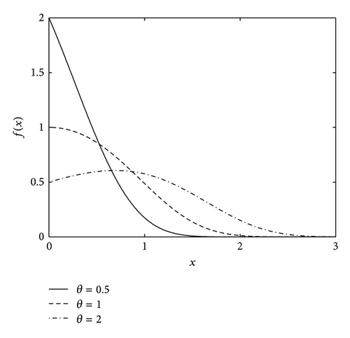
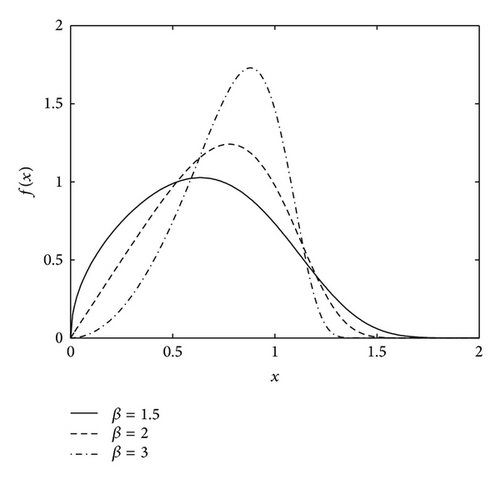
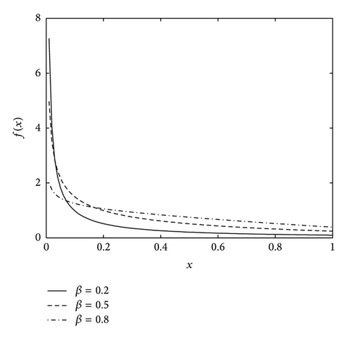
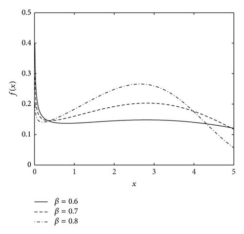
The failure rate function is , and , x > 0, thus λ(x) has a bathtub-shaped with achieving a minimum value at x = ((1 − β)/β)1/β when 0 < β < 1, and is increasing when β ≥ 1. Figure 2 illustrates λ(x) with various values of β and θ. Since the bottom of bathtub is the steady stage of failure rate function, it corresponds to the regular working stage of products and is very important for the practical application. To describe the length of time for working stage, we first give the definition of bathtub bottom width in the following.
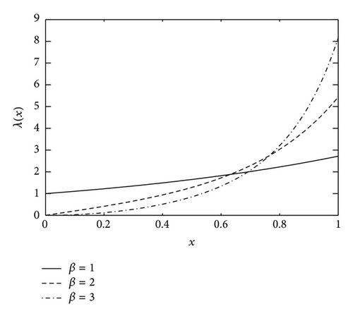
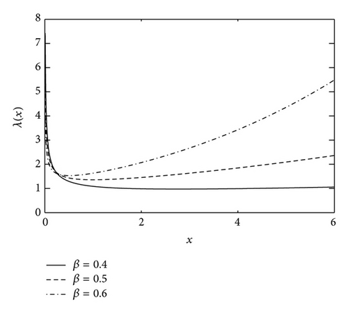
Definition 2. Suppose that a random variable X follows a bathtub-shaped failure rate function λ(x) with achieving the minimum at x0. For a given (bathtub height) ɛ > 0 and two roots x1, x2 of the equation λ(x) − λ(x0) = ɛ with x1 < x0 < x2, define the difference l(ɛ) = x2 − x1 as the bathtub bottom width of the given precision ɛ.
For CZM(β, θ) distribution, we have the following property of the bottom width for the failure rate function.
Theorem 3. For CZM(β, θ) with 0 < β < 1 and the bathtub-shaped failure rate function λ(x), then given ɛ > 0, the bathtub bottom width l(ɛ) is increasing for θ.
Proof. Since λ(x) has a bathtub-shaped for 0 < β < 1, given ɛ > 0, there are two roots x1 < x2 of the equation λ(x) − λ(x0) = ɛ with x0 = ((1 − β)/β)1/β. Taking derivative of the equation λ(x) − λ(x0) = ɛ with respect to θ, we have . Let , obviously g(x1) < 0 < g(x2) since x1 < x0 < x2. Thus, we obtain ∂l(ɛ)/∂θ = ∂(x2 − x1)/∂θ = (ɛ/β)[g(x2) − g(x1)] > 0. The theorem follows.
Given ɛ = 0.1,0.01,0.001,0.0001, and under various values of distribution parameters, the results of the bottom width are listed in Table 1, in which one can see that the width l(ɛ) is increasing for θ, on the contrary, l(ɛ) is decreasing for β.
| β = 0.5 | θ = 0.5 | |||||||
|---|---|---|---|---|---|---|---|---|
| ε | θ | x1 | x2 | l(ε) = x2 − x1 | β | x1 | x2 | l(ε) = x2 − x1 |
| 0.1 | 0.5 | 0.5696 | 1.6729 | 1.1033 | 0.3 | 5.7180 | 44.6868 | 38.9688 |
| 1 | 0.4475 | 2.0322 | 1.5847 | 0.5 | 0.5696 | 1.6729 | 1.1033 | |
| 2 | 0.3172 | 2.6219 | 2.3047 | 0.8 | 0.0867 | 0.3216 | 0.2349 | |
| 0.01 | 0.5 | 0.8404 | 1.1841 | 0.3437 | 0.3 | 12.0165 | 23.3669 | 11.3504 |
| 1 | 0.7810 | 1.2679 | 0.4869 | 0.5 | 0.8404 | 1.1841 | 0.3437 | |
| 2 | 0.7034 | 1.3943 | 0.6909 | 0.8 | 0.1428 | 0.2163 | 0.0734 | |
| 0.001 | 0.5 | 0.9470 | 1.0555 | 0.1085 | 0.3 | 15.1556 | 18.7121 | 3.5565 |
| 1 | 0.9257 | 1.0792 | 0.1535 | 0.5 | 0.9470 | 1.0555 | 0.1085 | |
| 2 | 0.8963 | 1.1135 | 0.2171 | 0.8 | 0.1655 | 0.1887 | 0.0232 | |
| 0.0001 | 0.5 | 0.9830 | 1.0173 | 0.0343 | 0.3 | 16.2962 | 17.4198 | 1.1236 |
| 1 | 0.9760 | 1.0245 | 0.0485 | 0.5 | 0.9830 | 1.0173 | 0.0343 | |
| 2 | 0.9662 | 1.0348 | 0.0686 | 0.8 | 0.1731 | 0.1805 | 0.0073 | |
For the purpose of estimation, we explore other characteristics of the distribution including finite moments. Finite moments guarantee the rationality for the moment-based estimation methods such as method of moments. We display our findings for the properties of CZM(β, θ) shown in Theorem 4 whose proof is provided in the Appendix.
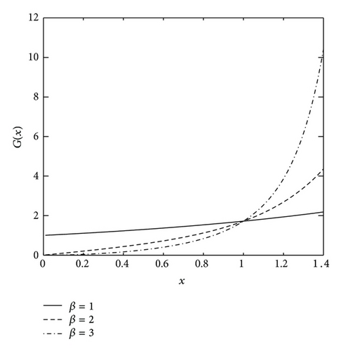
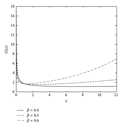
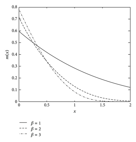
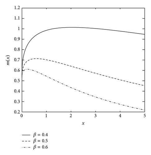
Theorem 4. Suppose X ~ CZM(β, θ). Then, (1) the moments exist; (2) the average failure rate G(x) = −(log(1 − F(x)))/x, x > 0 is increasing for β ≥ 1 and has a bathtub-shaped (concave-up) for 0 < β < 1; (3) the average remaining lifetime function , x > 0 is decreasing for β ≥ 1, and unimodal for 0 < β < 1.
Not surprisingly, there is a similar characteristic for the failure rate λ(x) and average failure rate G(x). Figures 3 and 4 illustrate the shapes of G(x) and m(x) with various values of β.
3. Estimation Methods
In this section, we discuss the estimation of parameters under type-II censored observational data. Suppose that n products whose lifetime follow CZM(β, θ) are placed on test and the test continues until predetermined r products fail with the ordered failure times x(1) ≤ x(2) ≤ ⋯≤x(r). We present the methods of point estimation for β, θ and the interval estimation only for the shape parameter β.
3.1. Maximum Likelihood Estimation
Lemma 5. Let with the constants a > 0, b > 0, then
- (1)
()
- (2)
For b > a > 0, ξ(β) is strictly increasing in β > 0.
3.2. Method of Moment Estimation
| n | r | 0.995 | 0.975 | 0.95 | 0.90 | 0.10 | 0.05 | 0.025 | 0.005 | |
|---|---|---|---|---|---|---|---|---|---|---|
| 10 | 8 | 0.1363 | 0.1437 | 0.1484 | 0.1545 | 0.2375 | 0.2592 | 0.2820 | 0.3361 | 0.1921 |
| 9 | 0.1251 | 0.1324 | 0.1370 | 0.1433 | 0.2255 | 0.2467 | 0.2692 | 0.3232 | 0.1803 | |
| 10 | 0.1178 | 0.1259 | 0.1311 | 0.1378 | 0.2367 | 0.2649 | 0.2927 | 0.3638 | 0.1819 | |
| 15 | 11 | 0.1022 | 0.1072 | 0.1104 | 0.1144 | 0.1628 | 0.1740 | 0.1851 | 0.2117 | 0.1365 |
| 12 | 0.0956 | 0.1005 | 0.1035 | 0.1073 | 0.1534 | 0.1640 | 0.1747 | 0.1998 | 0.1285 | |
| 13 | 0.0902 | 0.0951 | 0.0980 | 0.1018 | 0.1473 | 0.1582 | 0.1692 | 0.1951 | 0.1227 | |
| 14 | 0.0862 | 0.0913 | 0.0944 | 0.0983 | 0.1461 | 0.1577 | 0.1695 | 0.1984 | 0.1202 | |
| 15 | 0.0841 | 0.0898 | 0.0933 | 0.0978 | 0.1585 | 0.1750 | 0.1922 | 0.2333 | 0.1250 | |
| 20 | 16 | 0.0740 | 0.0775 | 0.0796 | 0.0824 | 0.1123 | 0.1189 | 0.1252 | 0.1403 | 0.0963 |
| 17 | 0.0708 | 0.0744 | 0.0765 | 0.0792 | 0.1088 | 0.1154 | 0.1217 | 0.1363 | 0.0930 | |
| 18 | 0.0684 | 0.0720 | 0.0742 | 0.0768 | 0.1071 | 0.1139 | 0.1204 | 0.1363 | 0.0908 | |
| 19 | 0.0665 | 0.0704 | 0.0726 | 0.0754 | 0.1081 | 0.1156 | 0.1230 | 0.1405 | 0.0905 | |
| 20 | 0.0661 | 0.0702 | 0.0728 | 0.0760 | 0.1185 | 0.1297 | 0.1410 | 0.1690 | 0.0952 | |
| 25 | 20 | 0.0605 | 0.0633 | 0.0649 | 0.0670 | 0.0885 | 0.0928 | 0.0970 | 0.1067 | 0.0770 |
| 21 | 0.0586 | 0.0613 | 0.0629 | 0.0649 | 0.0861 | 0.0905 | 0.0948 | 0.1040 | 0.0748 | |
| 22 | 0.0568 | 0.0596 | 0.0612 | 0.0632 | 0.0846 | 0.0890 | 0.0933 | 0.1031 | 0.0732 | |
| 23 | 0.0555 | 0.0584 | 0.0600 | 0.0620 | 0.0842 | 0.0890 | 0.0937 | 0.1042 | 0.0723 | |
| 24 | 0.0544 | 0.0575 | 0.0593 | 0.0614 | 0.0857 | 0.0911 | 0.0964 | 0.1095 | 0.0727 | |
| 25 | 0.0546 | 0.0580 | 0.0600 | 0.0625 | 0.0942 | 0.1022 | 0.1102 | 0.1312 | 0.0769 | |
| 30 | 24 | 0.0513 | 0.0536 | 0.0549 | 0.0565 | 0.0729 | 0.0762 | 0.0792 | 0.0860 | 0.0642 |
| 25 | 0.0499 | 0.0522 | 0.0534 | 0.0550 | 0.0711 | 0.0744 | 0.0774 | 0.0841 | 0.0626 | |
| 26 | 0.0487 | 0.0510 | 0.0522 | 0.0538 | 0.0699 | 0.0732 | 0.0763 | 0.0832 | 0.0614 | |
| 27 | 0.0477 | 0.0499 | 0.0512 | 0.0528 | 0.0691 | 0.0725 | 0.0758 | 0.0828 | 0.0605 | |
| 28 | 0.0469 | 0.0492 | 0.0505 | 0.0521 | 0.0693 | 0.0729 | 0.0762 | 0.0837 | 0.0602 | |
| 29 | 0.0465 | 0.0489 | 0.0503 | 0.0521 | 0.0710 | 0.0752 | 0.0792 | 0.0883 | 0.0609 | |
| 30 | 0.0466 | 0.0495 | 0.0511 | 0.0531 | 0.0779 | 0.0842 | 0.0906 | 0.1068 | 0.0645 | |
Furthermore, using this pivotal quantity, the 100 × (1 − α)% confidence interval for β is constructed from the roots of the equation a(n, r) = c with c the lower and upper (α/2)th quantiles under various settings of (n, r) in Table 2.
3.3. Inverse Method of Moment Estimation
To determine what value of k, in general, results in the optimal for Wu’s methods, we conduct a simulation study under various settings of (n, r). We only show the results for Wu’s exact interval since similar findings were obtained for Wu’s approximated method. We consider 3 ≤ k ≤ r − 3 to ensure the variance existence of F2(r−k),2k and its symmetry F2k,2(r−k). We choose the true values of parameters β = 1, θ = 1 and significance level α = 0.05 and calculate the interval estimations of parameter β based on 1000 Monte-Carlo simulations. The average upper and lower limits, average interval widths, and coverage probabilities are shown in Table 3, in which the least average interval width occurs at k = [r/3], where [·] is the greatest integer function. Thus it seems that the shortest interval is achieved when the sampling distribution is close to symmetric as much as possible.
| n | r | k | Average | Average | Average | Coverage |
|---|---|---|---|---|---|---|
| Lower limit | Upper limit | Interval width | Probability | |||
| 10 | 8 | 3 | 0.4016 | 2.6205 | 2.2189 | 0.956 |
| 4 | 0.3626 | 2.7726 | 2.4100 | 0.951 | ||
| 5 | 0.3293 | 3.3279 | 2.9986 | 0.961 | ||
| 9 | 3 | 0.4493 | 2.3191 | 1.8699 | 0.953 | |
| 4 | 0.4183 | 2.3419 | 1.9237 | 0,951 | ||
| 5 | 0.4190 | 2.7233 | 2.3043 | 0.942 | ||
| 15 | 13 | 3 | 0.5218 | 2.0465 | 1.5247 | 0.951 |
| 4 | 0.5113 | 2.0149 | 1.5036 | 0.946 | ||
| 5 | 0.5113 | 2.0591 | 1.5478 | 0.945 | ||
| 14 | 3 | 0.5350 | 1.9170 | 1.3820 | 0.951 | |
| 4 | 0.5267 | 1.8683 | 1.3415 | 0.956 | ||
| 5 | 0.5238 | 1.8768 | 1.3530 | 0.968 | ||
| 20 | 16 | 4 | 0.5443 | 1.9095 | 1.3652 | 0.951 |
| 5 | 0.5324 | 1.8901 | 1.3577 | 0.956 | ||
| 6 | 0.5350 | 1.9469 | 1.4120 | 0.954 | ||
| 7 | 0.5248 | 1.9774 | 1.4526 | 0.954 | ||
| 17 | 4 | 0.5576 | 1.8412 | 1.2836 | 0.955 | |
| 5 | 0.5490 | 1.8199 | 1.2709 | 0.951 | ||
| 6 | 0.5599 | 1.8739 | 1.3140 | 0.953 | ||
| 7 | 0.5420 | 1.8670 | 1.3250 | 0.962 | ||
| 18 | 5 | 0.5759 | 1.7837 | 1.2078 | 0.945 | |
| 6 | 0.5658 | 1.7607 | 1.1948 | 0.956 | ||
| 7 | 0.5673 | 1.7889 | 1.2216 | 0.943 | ||
| 8 | 0.5615 | 1.8075 | 1.2460 | 0.957 | ||
| 25 | 20 | 5 | 0.5833 | 1.7904 | 1.2071 | 0.951 |
| 6 | 0.5726 | 1.7644 | 1.1918 | 0.942 | ||
| 7 | 0.5838 | 1.8197 | 1.2359 | 0.951 | ||
| 8 | 0.5695 | 1.8198 | 1.2503 | 0.962 | ||
| 21 | 6 | 0.5934 | 1.7386 | 1.1452 | 0.944 | |
| 7 | 0.5854 | 1.7279 | 1.1425 | 0.946 | ||
| 8 | 0.5749 | 1.7237 | 1.1488 | 0.950 | ||
| 9 | 0.5810 | 1.7754 | 1.1944 | 0.951 | ||
| 22 | 6 | 0.6034 | 1.6876 | 1.0842 | 0.951 | |
| 7 | 0.5974 | 1.6753 | 1.0779 | 0.949 | ||
| 8 | 0.5910 | 1.6730 | 1.0820 | 0.949 | ||
| 9 | 0.5925 | 1.6984 | 1.1060 | 0.947 | ||
| 30 | 25 | 7 | 0.6201 | 1.6580 | 1.0378 | 0.952 |
| 8 | 0.6097 | 1.6447 | 1.0350 | 0.946 | ||
| 9 | 0.6080 | 1.6520 | 1.0439 | 0.950 | ||
| 10 | 0.6084 | 1.6730 | 1.0646 | 0.954 | ||
| 26 | 7 | 0.6301 | 1.6321 | 1.0020 | 0.944 | |
| 8 | 0.6219 | 1.6100 | 0.9881 | 0.951 | ||
| 9 | 0.6193 | 1.6158 | 0.9965 | 0.946 | ||
| 10 | 0.6166 | 1.6181 | 1.0016 | 0.958 | ||
| 27 | 8 | 0.6389 | 1.5909 | 0.9520 | 0.945 | |
| 9 | 0.6303 | 1.5768 | 0.9465 | 0.955 | ||
| 10 | 0.6324 | 1.5931 | 0.9607 | 0.948 | ||
| 11 | 0.6298 | 1.5955 | 0.9657 | 0.947 | ||
4. Simulation Study
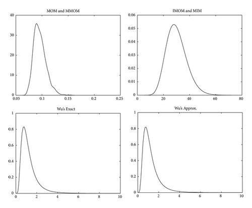
We investigate the precisions of presented point and interval estimation methods by Monte-Carlo simulations. We choose the true values of parameters β = 1, θ = 1, under which the density curve is shown in Figure 1(a), whose time scale is approximately 0 to 2. We generate 1000 random samples for each case of (n, r) in Table 4. The range of sample values is somehow related to the settings of (n, r). For example, the range of r = 8 observed values is 0.051 to 0.981 under n = 10, r = 8, while they are 0.0284 to 1.362 for n = 20, r = 18, and 0.018 and 1.483 for n = 30, r = 30. The point estimates of parameters β, θ for the 1000 generated samples under each case of (n, r) are calculated. Table 4 lists the mean and mean square error (MSE) of these estimates, among which MIM consistently produces the smallest MSE for the estimates and interestingly performs better than MLE under moderate sample size. To make more comparison, we also computed MOM estimates based on Wu’s exact quantity by setting up the equations through the first moments of , k = 1,2, …, r − 1. The least MSE occurs at k = [r/3] as well, and it lies (not shown in the table) between MSEs of MMOM and IMOM, so is larger than MIM’s. The 95% confidence intervals for β are also computed based on these simulated samples. The average upper and lower limits, average interval width and coverage probability are shown in Table 5, where Wu’s exact method in (12) selects the optimal interval estimation with k = [r/3]. It can be seen that MIM quantity in (9) produces the shortest average width of interval as well as least MSE for point estimation. We also did simulation studies under various settings of parameter values, including the case of bathtub-shape failure rate with 0 < β < 1. Similar results are obtained, showing that MIM approach consistently outperforms the other methods for both point and interval estimations (summary tables are not shown). The reason is that the log-scale expressed MIM quantity possesses less variability or its distribution is closer to symmetry than the distributions of other pivotal quantities. To illustrate this point, the density curves with n = 20, r = 16 of the four applied pivotal quantities: MOM, MIM, and Wu’s exact and approx. were shown in Figure 5, where the skewnesses of these distributions are 1.0878, 0.5164, 3.5058, and 3.5156, respectively, indicating the distribution of MIM pivot (whose skewness is 0.5164) is closest to symmetry.
| n | r | MLE | MOM | MMOM | IMOM | MIM | |||||
|---|---|---|---|---|---|---|---|---|---|---|---|
| Mean | MSE | Mean | MSE | Mean | MSE | Mean | MSE | Mean | MSE | ||
| 10 | 8 | 1.3251 | 0.4554 | 1.5849 | 1.0819 | 1.2588 | 0.4836 | 1.1701 | 0.3111 | 1.0034 | 0.2089 |
| 0.8921 | 0.1787 | 0.7928 | 0.2181 | 0.9077 | 0.1686 | 0.9427 | 0.1575 | 1.0073 | 0.1378 | ||
| 9 | 1.2712 | 0.3197 | 1.4863 | 0.7610 | 1.2325 | 0.3735 | 1.1225 | 0.2122 | 0.9882 | 0.1534 | |
| 0.9241 | 0.1555 | 0.8650 | 0.1889 | 0.9260 | 0.1477 | 0.9604 | 0.1452 | 0.9948 | 0.1214 | ||
| 10 | 1.1985 | 0.1949 | 1.3882 | 0.5076 | 1.1983 | 0.2675 | 1.0959 | 0.1413 | 0.9873 | 0.1082 | |
| 0.9933 | 0.1416 | 0.9883 | 0.1848 | 0.9879 | 0.1493 | 1.0005 | 0.1231 | 1.0088 | 0.1019 | ||
| 15 | 12 | 1.1955 | 0.1955 | 1.3323 | 0.3511 | 1.1466 | 0.1862 | 1.0893 | 0.1334 | 0.9907 | 0.1037 |
| 0.9197 | 0.1146 | 0.8448 | 0.1350 | 0.9305 | 0.1090 | 0.9704 | 0.1023 | 1.0107 | 0.0937 | ||
| 13 | 1.1565 | 0.1576 | 1.2694 | 0.2795 | 1.1167 | 0.1622 | 1.0744 | 0.1209 | 0.9878 | 0.0975 | |
| 0.9515 | 0.1028 | 0.9002 | 0.1180 | 0.9567 | 0.0984 | 0.9746 | 0.0929 | 1.0016 | 0.0837 | ||
| 14 | 1.1349 | 0.1215 | 1.2318 | 0.2377 | 1.1073 | 0.1404 | 1.0650 | 0.0798 | 0.9887 | 0.0655 | |
| 0.9629 | 0.0963 | 0.9346 | 0.1099 | 0.9642 | 0.0931 | 0.9784 | 0.0793 | 0.9944 | 0.0704 | ||
| 15 | 1.1200 | 0.0923 | 1.2292 | 0.2030 | 1.1257 | 0.1316 | 1.0525 | 0.0682 | 0.9858 | 0.0579 | |
| 0.9853 | 0.0867 | 0.9814 | 0.1068 | 0.9832 | 0.0891 | 0.9906 | 0.0808 | 0.9960 | 0.0715 | ||
| 20 | 17 | 1.1305 | 0.1007 | 1.2089 | 0.1668 | 1.0958 | 0.1048 | 1.0673 | 0.0804 | 1.0023 | 0.0669 |
| 0.9503 | 0.0732 | 0.9069 | 0.0836 | 0.9569 | 0.0716 | 0.9717 | 0.0676 | 0.9940 | 0.0625 | ||
| 18 | 1.1028 | 0.0834 | 1.1752 | 0.1409 | 1.0781 | 0.0938 | 1.0492 | 0.0601 | 0.9905 | 0.0516 | |
| 0.9621 | 0.0702 | 0.9287 | 0.0785 | 0.9629 | 0.0686 | 0.9836 | 0.0662 | 0.9991 | 0.0608 | ||
| 19 | 1.0948 | 0.0682 | 1.1685 | 0.1215 | 1.0867 | 0.0841 | 1.0450 | 0.0524 | 0.9915 | 0.0456 | |
| 0.9716 | 0.0575 | 0.9502 | 0.0659 | 0.9691 | 0.0581 | 0.9857 | 0.0637 | 0.9953 | 0.0582 | ||
| 20 | 1.0921 | 0.0599 | 1.1683 | 0.1197 | 1.0978 | 0.0854 | 1.0371 | 0.0519 | 0.9892 | 0.0463 | |
| 0.9974 | 0.0614 | 0.9938 | 0.0707 | 0.9954 | 0.0625 | 1.0030 | 0.0574 | 1.0061 | 0.0525 | ||
| 25 | 22 | 1.0801 | 0.0626 | 1.1397 | 0.0979 | 1.0597 | 0.0692 | 1.0399 | 0.0528 | 0.9925 | 0.0468 |
| 0.9624 | 0.0508 | 0.9294 | 0.0576 | 0.9631 | 0.0508 | 0.9824 | 0.0495 | 0.9968 | 0.0463 | ||
| 23 | 1.0782 | 0.0524 | 1.1362 | 0.0852 | 1.0644 | 0.0607 | 1.0358 | 0.0459 | 0.9917 | 0.0411 | |
| 0.9746 | 0.0499 | 0.9507 | 0.0561 | 0.9741 | 0.0502 | 0.9848 | 0.0468 | 0.9952 | 0.0437 | ||
| 24 | 1.0789 | 0.0523 | 1.1273 | 0.0823 | 1.0656 | 0.0609 | 1.0489 | 0.0454 | 1.0075 | 0.0398 | |
| 0.9795 | 0.0486 | 0.9649 | 0.0531 | 0.9781 | 0.0480 | 0.9876 | 0.0463 | 0.9940 | 0.0429 | ||
| 25 | 1.0634 | 0.0405 | 1.1251 | 0.0754 | 1.0725 | 0.0572 | 1.0267 | 0.0397 | 0.9893 | 0.0366 | |
| 1.0019 | 0.0464 | 0.9994 | 0.0531 | 1.0007 | 0.0481 | 1.0136 | 0.0423 | 1.0158 | 0.0395 | ||
| 30 | 27 | 1.0679 | 0.0445 | 1.1110 | 0.0683 | 1.0494 | 0.0508 | 1.0310 | 0.0387 | 0.9934 | 0.0351 |
| 0.9775 | 0.0449 | 0.9536 | 0.0483 | 0.9775 | 0.0441 | 0.9831 | 0.0409 | 0.9933 | 0.0387 | ||
| 28 | 1.0649 | 0.0399 | 1.1101 | 0.0617 | 1.0556 | 0.0467 | 1.0293 | 0.0342 | 0.9939 | 0.0312 | |
| 0.9755 | 0.0408 | 0.9590 | 0.0451 | 0.9756 | 0.0412 | 0.9846 | 0.0389 | 0.9922 | 0.0367 | ||
| 29 | 1.0606 | 0.0379 | 1.0957 | 0.0572 | 1.0492 | 0.0451 | 1.0386 | 0.0352 | 1.0052 | 0.0317 | |
| 0.9845 | 0.0404 | 0.9746 | 0.0425 | 0.9839 | 0.0395 | 0.9860 | 0.0370 | 0.9909 | 0.0349 | ||
| 30 | 1.0549 | 0.0315 | 1.1104 | 0.0593 | 1.0677 | 0.0464 | 1.0159 | 0.0298 | 0.9853 | 0.0282 | |
| 1.0014 | 0.0373 | 0.9980 | 0.0421 | 0.9992 | 0.0389 | 1.0046 | 0.0368 | 1.0065 | 0.0348 | ||
| n | r | Wu’s exact | MOM pivot | MIM pivot |
|---|---|---|---|---|
| (coverage probability) | (coverage probability) | (coverage probability) | ||
| 10 | 8 | 2.2189 (0.956) | 2.4262 (0.962) | 1.6850 (0.951) |
| 9 | 1.8699 (0.953) | 2.0865 (0.960) | 1.4650 (0.954) | |
| 10 | 1.5398 (0.954) | 1.8407 (0.957) | 1.2372 (0.952) | |
| 15 | 12 | 1.5989 (0.946) | 1.6231 (0.958) | 1.2542 (0.956) |
| 13 | 1.5036 (0.946) | 1.5421 (0.946) | 1.1714 (0.955) | |
| 14 | 1.3415 (0.956) | 1.3138 (0.949) | 1.0601 (0.953) | |
| 15 | 1.1966 (0.956) | 1.2606 (0.951) | 0.9537 (0.949) | |
| 20 | 16 | 1.3577 (0.956) | 1.2771 (0.952) | 1.0681 (0.950) |
| 17 | 1.2709 (0.951) | 1.2150 (0.961) | 1.0018 (0.963) | |
| 18 | 1.1948 (0.956) | 1.1268 (0.953) | 0.9360 (0.955) | |
| 19 | 1.1022 (0.950) | 1.0185 (0.943) | 0.8821 (0.960) | |
| 20 | 1.0075 (0.950) | 1.0016 (0.947) | 0.8100 (0.950) | |
| 25 | 20 | 1.1918 (0.942) | 1.0922 (0.943) | 0.9306 (0.948) |
| 21 | 1.1425 (0.946) | 1.0411 (0.959) | 0.8896 (0.950) | |
| 22 | 1.0779 (0.949) | 0.9787 (0.954) | 0.8455 (0.953) | |
| 23 | 1.0166 (0.945) | 0.9380 (0.954) | 0.8025 (0.955) | |
| 24 | 0.9526 (0.946) | 0.8832 (0.948) | 0.7578 (0.960) | |
| 25 | 0.8863 (0.951) | 0.8644 (0.943) | 0.7149 (0.953) | |
| 30 | 24 | 1.0806 (0.950) | 0.9752 (0.954) | 0.8420 (0.949) |
| 25 | 1.0350 (0.946) | 0.9187 (0.945) | 0.8086 (0.956) | |
| 26 | 0.9881 (0.951) | 0.8959 (0.951) | 0.7785 (0.956) | |
| 27 | 0.9465 (0.955) | 0.8407 (0.955) | 0.7454 (0.961) | |
| 28 | 0.9022 (0.956) | 0.8212 (0.945) | 0.7150 (0.951) | |
| 29 | 0.8543 (0.943) | 0.7807 (0.941) | 0.6792 (0.954) | |
| 30 | 0.8039 (0.955) | 0.7714 (0.947) | 0.6438 (0.948) | |
5. Illustrative Examples
In this section, we apply the presented approaches on two examples to compare the efficiency of estimation methods.
Example 6. Wu et al. [11] presented a complete failure hour of 18 electronic equipments: 5, 11, 21, 31, 46, 75, 98, 122, 145, 165, 195, 224, 245, 293, 321, 330, 350, and 420. Xie et al. [18] showed that the data had bathtub failure rate function, so we fit this dataset by CZM(β, θ) to obtain the estimation results summarized in Table 6. In this case of relatively small sample size n = 18, MIM should yield reliable estimates based on the simulation study. From the results of the 95% confidence interval for β, one may see that the shortest Wu’s exact interval occurs at k = 7, a little narrower than that of Wu’s exact with k = [18/3] = 6. This indicates that maybe the data slightly deviate from CZM(β, θ). Although Wu’s approx. gives a shorter width than that from Wu’s exact, it is a large-sample based approach whose coverage probability might not be the same as the nominal under the small sample size. Overall, MIM pivot produces the shortest interval among all the methods in accordance with the findings in the simulation study.
| Parameter | MLE | MOM | MMOM | IMOM | MIM |
|---|---|---|---|---|---|
| β | 0.2893 | 0.3102 | 0.3005 | 0.2806 | 0.2741 |
| θ | 100.4048 | 189.7327 | 139.5206 | 78.9727 | 66.6931 |
| Approach | 95% confidence interval for β | Length | |||
| Chen’s (Wu’s exact k = 1) | (0.1986, 0.3697) | 0.1771 | |||
| Wu’s exact (k = 7) | (0.2106, 0.3299) | 0.1193 | |||
| Wu’s exact (k = 6) | (0.2066, 0.3261) | 0.1195 | |||
| Wu’s approximated (k = 5) | (0.2122, 0.3220) | 0.1098 | |||
| MOM pivot | (0.2304, 0.3640) | 0.1336 | |||
| MIM pivot | (0.2237, 0.3260) | 0.1023 | |||
Example 7. Chen [6] presented a type-II censoring data of n = 15 samples from CZM(0.5,50), in which there was r = 11 complete failures: 0.29, 1.44, 8.38, 8.66, 10.20, 11.04, 13.44, 14.37, 17.05, 17.13, and 18.35. Notably, since β = 0.5 < 1, the data was from the distribution with a bathtub-shaped failure rate. The estimation results by the proposed methods are shown in Table 7, where we notice that some methods perform better than MIM (particularly for the estimation of β), but not significantly. Despite only 11 complete failures out of 15 samples used in the estimation, MIM still yields a comparable point estimates. For the 95% confidence interval of β, Wu’s exact and approx. with k = [11/3] = 3 produce the least lengths among all intervals for k = 1,2, …, 10. Also MIM pivot gives the shortest length of interval as expected. In summary, although it is an example of bathtub-shaped failure rate, the results are in accordance with the findings in the simulation study, where the comparisons are based on the data generated from a nonbathtub shaped failure rate function with β = 1.
| Parameter | MLE | MOM | MMOM | IMOM | MIM |
|---|---|---|---|---|---|
| β | 0.5068 | 0.5471 | 0.5071 | 0.4648 | 0.4584 |
| θ | 63.8939 | 102.2165 | 64.7495 | 40.3122 | 41.5428 |
| Approach | 95% confidence interval for β | Length | |||
| Chen’s (Wu’s exact k = 1) | (0.1900, 0.6200) | 0.4300 | |||
| Wu’s exact (k = 3) | (0.3783, 0.7049) | 0.3266 | |||
| Wu’s approximated (k = 3) | (0.3803, 0.6957) | 0.3154 | |||
| MOM pivot | (0.3013, 0.6492) | 0.3479 | |||
| MIM pivot | (0.2955, 0.5998) | 0.3043 | |||
6. Conclusions
In this paper, we consider the parameter inference for a two-parameter life distribution. We present five point estimations and three interval estimations for the parameter of interest. Through the Monte-Carlo simulation technique, we determined a mechanism to obtain the optimal interval estimation originally proposed by Wu et al. [11]. The performance of the methods were assessed by a comparison of estimation precisions, and it showed that the MIM pivotal quantity with a log-scale expression leads to a relative effectiveness of the estimation under moderate sample size. This indicated that the quantity has less variability or its distribution is closer to symmetry. We applied the methods to two datasets and demonstrated the efficiency of MIM estimation method.
Conflict of Interests
The authors declare that there is no conflict of interests regarding the publication of this paper.
Acknowledgments
Wang and Xu’s work was supported by the Grants from Innovation Program of Shanghai Municipal Education Commission (14YZ080, 14ZZ155). Wang’s work was also supported by Shanghai Normal University SK201306. Sha’s work was partially supported by NSF CMMI-0654417, and NIH NIMHD-8G12MD007592.
Appendix
Proof of Lemma 1. (1) When β = 1, we have f′(x) = (1 − ex/θ)/θexp(x + (1 − ex)/θ). Obviously, f′(x) < 0 when 0 < θ ≤ 1, and f(x) is unimodal at x0 = logθ when θ > 1.
For β ≠ 1, first we have
(2) When β > 1, we know limx→0g(x) = (β − 1)θ > 0, so there exists a unique positive root x0 of g(x) = 0. Therefore, g(x) > 0, and then f′(x) > 0 in 0 < x < x0, but g(x) < 0, then f′(x) < 0 in x > x0, as a result f(x) is unimodal.
(3) When 0 < β < 1, then limx→0g(x) = (β − 1)θ < 0, limx→+∞g(x) = −∞. Note that limx→0f(x) = +∞, limx→+∞f(x) = 0. (i) for 0 < θ ≤ 1, then we have g′(x) < 0, and so g(x) < 0, thus f′(x) < 0, that is, f(x) is decreasing; (ii) for θ > 1, (a) if g(x1) ≤ 0, then we have g(x) ≤ 0, f′(x) ≤ 0, that is, f(x) is decreasing; (b) if g(x1) > 0, then there are two positive roots x01, x02 of g(x) = 0 with 0 < x01 < x1 < x02. First for 0 < x < x01, we have g(x) < 0, f′(x) < 0, and so f(x) is decreasing. Secondly for x01 < x < x02, we have g(x) > 0, f′(x) > 0, and so f(x) is increasing. Finally for x > x02, we have g(x) < 0, f′(x) < 0, and so f(x) is decreasing.
The following mathematical result will be used in the proof of Theorem 4.
Lemma A.1 (see [19].)Let g(x) be a nonnegative function at [a, +∞) and integrable at [a, b] for any b > a. If limx→+∞((logg(x))/logx) = p, then is convergent for −∞ ≤ p < −1, and divergent for −1 < p ≤ +∞.
Proof of Theorem 4. (1) The kth moment is
(2) , so . Setting the function , we have limx→0g(x) = 0, limx→+∞g(x) = +∞, and , then
- (i)
when β ≥ 1, we have g′(x) > 0, then g(x) > 0, G′(x) > 0, that is, G(x) is increasing;
- (ii)
when 0 < β < 1, let x0 = ((1 − β)/β)1/β, and then we have g′(x) < 0 in 0 < x < x0 and g′(x) > 0 in x > x0. Also g(x0) = 1 − βe(1 − β)/β < 0, therefore, there exists a root x1 of g(x) = 0 with x1 > x0 > 0. Then we have g(x) < 0, G′(x) < 0, so G(x) is decreasing in 0 < x < x1, and g(x) > 0, G′(x) > 0, so G(x) is increasing in x > x1. That is G(x) is a bathtub-shape (concave-up) function.
(3) , then
- (i)
When β > 1, we have g′(x) > 0, limx→0g(x) = −∞, limx→+∞g(x) = 0, so g(x) < 0, and thus m′(x) < 0.
- (ii)
When β = 1, we have g′(x) = θe−xexp((1 − ex)/θ) > 0, , limx→+∞g(x) = 0, so g(x) < 0, m′(x) < 0.
- (iii)
When 0 < β < 1, with x0 = ((1 − β)/β)1/β, we get g′(x) < 0 in 0 < x < x0 and g′(x) > 0 in x > x0. Also , limx→+∞g(x) = 0, and = since (1 − β)t−β − β < 0 in t > x0. Thus, there is a unique root x1 of g(x) = 0 with 0 < x1 < x0, so that g(x) > 0, m′(x) > 0 in 0 < x < x1 and g(x) < 0, m′(x) < 0 in x > x1. That is, m(x) is unimodal.
Proof of Lemma 5. The proof of (1) is clear, therefore we only show the proof for (2). Chen [6] gave a proof, but it was wrong since in general two increasing functions, say f(x), g(x) can not guarantee the product f(x)g(x) being increasing unless both f(x) and g(x) are positive functions. Here we give the correct proof as follows.
Since , then
(i) for x ≥ 1, obviously logx ≥ 0, and so g(x) > 0.
(ii) for 0 < x < 1, first k + 1 + xlogx ≥ 2 + xlogx for k ≥ 1. Additionally, we know g1(x) = 2 + xlogx is a concave-up function in 0 < x < 1 with achieving minimum value g1(e−1) = 2 − e−1 > 0, so g1(x) > 0, and then g(x) > 0 in 0 < x < 1.
In conclusion, we obtain g(x) > 0 in x > 0, and so f′(x) > 0, that is, f(x) is strictly increasing in x > 0. The lemma follows.
Proof of Uniqueness of MLE. We denote the left side of the second equation in (4) as H(β). It is obvious that limβ→0H(β) = −∞. Now we consider limβ→+∞H(β) for various cases by using Lemma 5.
(1) When x(r) ≤ 1, then x(i) < 1, i = 1,2, …, r − 1. Note that
(2) When x(r) > 1, note that
In conclusion, H(β) is increasing and limβ→0H(β) = −∞, limβ→+∞H(β) > 0, thus the equation H(β) = 0 must have a unique positive root.
Proof of Uniqueness of MOM. Let , then
Additionally, on the one hand, , and on the other hand


