We develop a cobweb model with discrete time delays that characterise the length of production cycle. We assume a market comprised of homogeneous producers that operate as adapters by taking the (expected) profit-maximising quantity as a target to adjust production and consumers with a marginal willingness to pay captured by an isoelastic demand. The dynamics of the economy is characterised by a one-dimensional delay differential equation. In this context, we show that (1) if the elasticity of market demand is sufficiently high, the steady-state equilibrium is locally asymptotically stable and (2) if the elasticity of market demand is sufficiently low, quasiperiodic oscillations emerge when the time lag (that represents the length of production cycle) is high enough.

1. Introduction

Time series of prices of nonstorable goods are observed on a daily basis and are subject to strong fluctuations, while production of such commodities requires a longer time period (for instance, from sowing to harvest with regard to agricultural ones). The cobweb model, originally developed by Kaldor [1] with linear supply and demand, (see also Ezekiel [2].) has been extensively investigated in a discrete time deterministic context (e.g., [3–8]). (For a stochastic version of a discrete time cobweb model see Brianzoni et al. [9].) It essentially served to explain the reasons why prices of commodities in the agricultural sector fluctuate over time. According to that model, farmers operate in a market where production must be chosen before prices are observed (i.e., there exists a time lag in supply). Producers’ choices, therefore, depend on prices they expect to prevail at harvest time. By assuming that farmers take the current price as an estimate of the expected price (static expectations), stability of the market equilibrium is shown to depend on relative elasticities of supply and demand. Assume that farmers plant wheat and corn at a certain date, and they are forced to sell their entire production. If they expect that the price of wheat will be high and that of corn low, they will plant a large amount of wheat in the future. Nevertheless, it is possible that market interactions between supply and demand (or, alternatively, other reasons related, for instance, to unexpected weather events and so on; see [9]) do cause a price for wheat lower than the expected one. As a consequence, producers’ decisions will be modified accordingly giving rise to price fluctuations. The traditional cobweb model with static expectations, therefore, represents a very useful tool for the analysis of price dynamics. However, only three different kinds of phenomena can be observed if supply and demand are linear: convergence towards the steady-state equilibrium, cycle of period two, and unbounded fluctuations.

The interest in the study of price dynamics has led Hommes [3] to extend the discrete time cobweb model by introducing adaptive expectations (Adaptive expectations have been introduced in the original cobweb model by Nerlove [10].) and nonlinear supply and demand curves. In his work, he showed that chaotic behaviours in prices can occur even if supply and demand are monotonic. (Artstein [11] and Jensen and Urban [12] found that chaotic price dynamics can arise also in the model with static expectations if either the supply curve or demand curve is nonmonotonic.) Subsequently, Gallas and Nusse [13] have deepened some mathematical properties of that model with adaptive expectations, while Mammana and Michetti [14, 15] have analysed the role of memory and expectations in such a context.

By considering quantity instead of price as the main variable, Onozaki et al. [4, 5] provided examples of the importance of behaviours other than rational expectations as a source of complex dynamics in the cobweb model. In particular, the former paper takes into account adaptive adjustments on the quantity produced instead of adaptive expectations on prices (as in [3]). With this behavioural rule, farmers partially adjust production in the direction of the best response (represented by the quantity that maximises expected profits). By assuming a nonlinear (monotonic) market demand, they showed—by using the Homoclinic Point Theorem—that topological chaos can occur in a model whose dynamics is characterised by a one-dimensional map. From an economic point of view, chaos occurs more likely the faster suppliers adjust production and the more inelastic the market demand is. The latter paper extends the former one by introducing behavioural heterogeneity of producers.

To capture in a better way the functioning of a market whose price fluctuations are observed on a daily basis, this paper extends Onozaki et al.’s [4] by considering a continuous time cobweb model with discrete time delays. The time delay is introduced to describe a specific aspect of agricultural commodity markets: the production cycle of nonstorable goods, in fact, is elapsed from sowing time to harvest time (see [16], for an analysis of a continuous time cobweb model with time delays). In this paper, we consider an economy with consumers whose marginal willingness to pay is determined by an isoelastic demand, and homogeneous farmers that face quadratic costs. Producers behave as adapters and take into account the profit maximising quantity as a target to adjust production. The dynamics of the economy is characterised by a single delay differential equation. In this context, we show that (1) if the elasticity of market demand is sufficiently high, the steady-state equilibrium is locally asymptotically stable (prices adequately react to clear the market) and (2) if the elasticity of market demand is sufficiently low, quasiperiodic oscillations emerge when the time lag (that represents the length of production cycle) is high enough.

The rest of the paper is organised as follows. Section 2 sets up the cobweb model with homogeneous producers that operate as adapters. Section 3 characterises local stability properties and local bifurcations of equilibria of the resulting one-dimensional delay differential equation. Section 4 studies stability properties and the direction of the Hopf bifurcation. Section 5 provides some numerical experiments to validate the theoretical results established in previous sections. Section 6 outlines the conclusions.

2. The Model

We consider a continuous time version with discrete time delays of the model developed by Onozaki et al. [4]. There exist n > 0 identical and competitive firms that operate in the agricultural sector. We assume that the technology of production requires a period of time τ to bring the production process to completion and get products to the market. The quantity that maximises the expected profit at time t is solution of the following problem referred at time t − τ:

()

where b > 0 is a constant parameter and p^e(t), q(t), and b[q(t)] ²/2 are the price expected at time t, the quantity of the agricultural good, and the quadratic cost function referred at time t, respectively. It is important to note that expectations on prices do appear in (1). This is because the price that will prevail at time t is not known at the time the maximisation problem of expected profits is referred; that is, t − τ. Assume now that producers have static expectations on prices; that is, p^e(t) = p(t − τ). Then, maximisation programme (1) gives

()

Let firms be (expected) profit maximisers and use the quantity that corresponds to maximum expected profits,

, as a target to adjust production choices. In particular, if the quantity produced at time t is smaller (resp., greater) than

, farmers will increase (resp., reduce) production. Then, we assume the following behavioural rule for production decisions of each single farmer:

()

where 0 < α < 1 is the speed of adjustment. This rule can be interpreted as a precautionary behaviour with respect to the evolution of the market price. (See Brock and Hommes [17], Bischi et al. [18, 19], Chiarella et al. [20], and Fanti et al. [21] for different behavioural rules of economic agents without rational expectations.)

Since there are n homogeneous firms, aggregate supply can easily be determined as follows:

()

With regard to consumers’ side, by following Fanti et al. [22], we assume the existence of a continuum of identical consumers whose preferences towards both the agricultural commodity y (whose price is p) and numeraire good w (whose price is normalised to one without loss of generality), produced by competitive firms, are represented by the following quasilinear utility function:

()

with

()

Here, 1/β is the constant demand elasticity and c > 0 represents the extent of market demand. The representative consumer maximises utility function (6) subject to budget constraint py + w = M, where M > 0 is the exogenous nominal income of the consumer (M is assumed to be sufficiently high to avoid the existence of corner solutions). This maximisation programme implies that the isoelastic inverse demand of good y is determined as follows:

()

Therefore, the market demand of the agricultural commodity at time t is the following:

()

Market equilibrium, therefore, implies that aggregate demand equals aggregate supply, that is, x(t) = y(t) for any t. Then, by using (2)–(8) we find the following delay differential equation that characterises the dynamics of the model: (See Haldane [23] for a pioneering contribution on the use of delay differential equations applied to a model of price dynamics.)

()

where x_d : = x(t − τ).

3. Existence of Equilibria and Local Bifurcations

The steady-state equilibrium of (9) satisfies x_d = x = x_* for all t so that the time derivative vanishes identically. It is immediate that equilibria of (9) coincide with those for τ = 0. Direct calculations show the existence of a unique positive equilibrium x_* such that

. Linearization of (9) in the neighbourhood of this equilibrium produces the following equation:

()

The corresponding characteristic equation therefore is

()

When there is no delay, that is, τ = 0 in (11), the characteristic equation becomes P(λ, 0) = λ + α + αβ = 0. Hence, x_* is locally asymptotically stable since λ = −α(1 + β) < 0.

Assume now that τ > 0 in (11). We will investigate location of the roots of the transcendental equation. First, we examine when this equation has zero or pure imaginary roots. Now, it is immediate that the former cannot occur.

Lemma 1. Let β > 1. The characteristic equation (11) associated with (9) has a pair of purely imaginary roots λ = ±iω₀ at a sequence of critical values τ_j, where

()

Proof. Let λ = iω be a root of the characteristic equation (11) where ω > 0. Substituting this in (11), separating real and imaginary parts of the resulting equation, we obtain the solution of (11) as follows:

()

This leads to

()

It is immediate to see that if β > 1 holds, then (15) has only one positive root. Next, from (14) one obtains the critical values τ_j by noting that −ω₀/α < 0.

Lemma 2. λ = iω₀ is a simple purely imaginary root of the characteristic equation (11) and all the other roots λ ≠ iω₀ satisfy λ ≠ imω₀ for any integer m.

Proof. If λ = iω₀ were not simple, that is, P(iω₀, τ_j) = P^′(iω₀, τ_j) = 0, then we would have 1 + ατ_j + iω₀τ_j = 0, which is a contradiction. In order to establish the last part of the lemma, let us suppose there exists a root λ_m such that P(λ_m, τ₀) = 0 and λ_m = imω₀, for some m ≠ 0, ±1. From (14), we get , namely, m² = 1. This completes the proof.

Lemma 3. The following transversality condition:

()

is satisfied.

Proof. Let λ(τ) = ν(τ) + iω(τ) denote the roots of (11) near τ_j satisfying the conditions ν(τ_j) = 0 and ω(τ_j) = ω₀. Differentiating the characteristic equation (11) with respect to τ, using (11), and solving for dλ/dτ term, we get

()

This gives

()

Hence, we have

()

The previous lemma implies that the root of characteristic equation (11) near τ_j crosses the imaginary axis from the left to the right as τ continuously varies from a number less than τ_j to one greater than τ_j by Rouché’s theorem.

Proposition 4. If τ ∈ [0, τ₀), all roots of (11) have negative real parts. If τ = τ₀, all roots of (11) except λ = ±iω₀ have negative real parts. If τ ∈ (τ_j, τ_j+1), for j = 0,1, 2, …, (11) has 2(j + 1) roots with positive real parts.

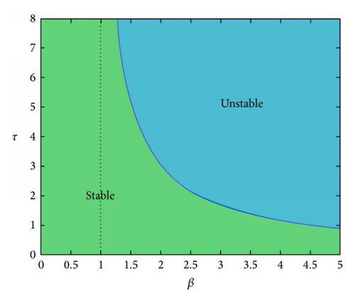
Summing up, we can state the following results (see Figure 1).

Details are in the caption following the image — **Figure 1**
Open in figure viewer PowerPoint

Stability and instability regions in (β, τ) space are depicted in green and blue, respectively. According to Theorem 5, on the left of the dotted line the equilibrium is locally asymptotically stable for any τ. Parameter set: α = 0.4, c = 0.77, n = 1, and b = 0.3.

Theorem 5. Let ω₀ and τ_j be defined as in (12) and (13), respectively. For (9), the following statements are true.

(1)
If β ≤ 1, the positive equilibrium x_* is locally asymptotically stable for all τ ≥ 0.
(2)
If β > 1, the positive equilibrium x_* is locally asymptotically stable for τ ∈ [0, τ₀) and unstable for τ > τ₀.
(3)
If β > 1, (9) undergoes a Hopf bifurcation at the positive equilibrium x_* when τ = τ_j, j = 0,1, 2, ….

4. Stability and Direction of the Hopf Bifurcation

In the previous section we have obtained conditions for Hopf bifurcation to occur when τ = τ_j, j = 0,1, 2, …. In this section we will study direction, local stability, and period of these periodic solutions bifurcating from equilibrium x_* at these critical values of τ. The method used here is based on the normal form and center manifold theory introduced by Hassard et al. [24]. Without loss of generality, we will investigate the critical value τ = τ₀ at which (9) undergoes a Hopf bifurcation from x_*. For convenience, let τ = τ₀ + μ,

. Then μ = 0 is the Hopf bifurcation value for (9). Setting u = x − x_*, then expanding (9) into first, second, third, and other higher-order terms at the trivial equilibrium gives

()

For

, let

()

By the Riesz representation theorem, there is a bounded variation function η(θ, μ) in θ ∈ [−τ₀, 0] such that

()

In fact, we can choose

()

where δ is the Dirac delta function. For

, we set

()

Then (20) can be rewritten as

()

where u_t = u(t + θ), for θ ∈ [−τ₀, 0]. For

, define

()

For

and

, using the bilinear form

()

we know that A^* and A = A(0) are adjoint operators. By the discussion in Section 3, we know that ±iω₀ are eigenvalues of A. Thus, they are eigenvalues of A^*. Clearly,

is an eigenvector of A corresponding to the eigenvalue iω₀, and

is an eigenvector of A^* corresponding to the eigenvalue −iω₀, where

()

Hence, we have 〈h^*, h〉 = 1 and

Using the same notations as in Hassard et al. [24], we first compute coordinates to describe the center manifold C₀ at μ = 0. Let u_t be the solution of (20) when μ = 0. Define

()

On the center manifold C₀, we have

, where

()

where z and

are local coordinates for the center manifold C₀ in the direction of h^* and

, respectively. For solution u_t ∈ C₀ of (25), since μ = 0, we have

()

where

()

Rewrite (31) as

()

where

()

By (29) and (31) we have

()

that is,

()

where

()

Note that

. Therefore, we get

()

From (34), using

and comparing coefficients, we obtain

()

Since there are W₁₁(−τ₀) and W₂₀(−τ₀) in g₂₁, we still need to compute them. From (36), we have

()

Hence, we find

()

On the other hand, on the center manifold,

()

Next, using (30) and (33) we derive another expression for

. Then a comparison with (36) leads to the equations:

()

From (25) and (36), it follows that

()

Hence,

()

where E₁ and E₂ are both real constants and can be determined by setting θ = 0 in

. In fact,

()

Now, (30) and (36) give

()

Substituting (47) into (46), we can calculate E₁ and E₂.

Based on the above analysis, we can see that each g_ij in (39) is determined. Thus, we can compute the following values:

()

It is well known that μ₂ determines the direction of the Hopf bifurcation: if μ₂ > 0 (resp., μ₂ < 0), then the Hopf bifurcation is supercritical (resp., subcritical) and the bifurcating periodic solutions exist for τ > τ₀ (resp., τ < τ₀); β₂ determines the stability of bifurcating periodic solutions: the bifurcating periodic solutions on the center manifold are stable (resp., unstable) if β₂ < 0 (resp., β₂ > 0); T₂ determines the period of the bifurcating periodic solutions: the period increases (resp., decreases) if T₂ > 0 (resp., T₂ < 0). From the discussion in Section 3 we know that Re{λ^′(τ₀)} > 0. Therefore, we have the following result.

Theorem 6. Let Re{C₁(0)} be given in (48). The direction of the Hopf bifurcation of (9) at equilibrium x_* when τ = τ₀ is supercritical (resp., subcritical) and the bifurcating periodic solutions on the center manifold are stable (resp., unstable) if Re{C₁(0)} < 0 (resp., Re{C₁(0)} > 0).

5. Numerical Simulations

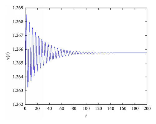
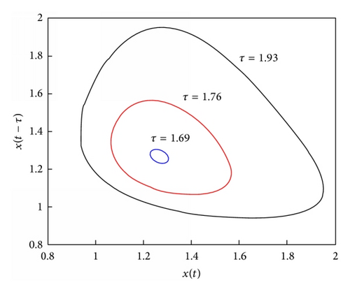
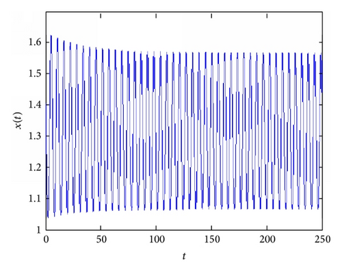
We now illustrate the theoretical results stated in previous sections by performing some numerical simulations. For this purpose, we fix the following parameter set: α = 0.4, β = 3, c = 0.77, n = 1, and b = 0.3 and let τ vary. With this parameter values, the steady-state equilibrium is x_*≃1.266 and the Hopf bifurcation occurs at τ₀≃1.689. When τ < τ₀ (but sufficiently high), the dynamics of the quantity produced by farmers are oscillatory and convergent towards the equilibrium (as shown in Figure 2). Just after the Hopf bifurcation value of τ, there exists an attracting closed invariant curve and then the dynamics of quantities show persistent oscillations. To this purpose, Figure 3 shows the dependency of the length of the diameter of the closed invariant curve on the time lag τ. In particular, the figure depicts three different closed invariant curves for three different values of τ, that is, τ = 1.69 (blue curve), τ = 1.76 (red curve), and τ = 1.93 (black curve). It clearly shows that the length of the diameter of the closed invariant curve increases with τ. This implies that when τ is sufficiently high (i.e., the length of productive cycle is large), the amplitude of fluctuations of quantities (and prices) may be relevant (see Figure 4).

6. Conclusions

This paper extended the discrete time cobweb model by Onozaki et al. [4] with discrete time delays that characterise the length of production cycle. The model economy consists of homogeneous farmers that behave as adapters and refer to the expected profit-maximising quantity (with static expectations) as the target to which production is directed; that is, producers partially adjust their output by moving towards the best response. “Such adjustment is a behavioral response to uncertainty and adjustment costs” [4, page 102]. In a discrete time framework, Onozaki et al. [4] showed that the model can generate topological and observable chaos by applying the Homoclinic Point Theorem. In a continuous time version of that model, we found that the size of time lag in production matters for the emergence of nonlinear dynamics. In particular, by means of Hassard techniques we characterise existence and stability properties of the Hopf bifurcation that occurs when the time delay is sufficiently high. After the supercritical Hopf bifurcation, quasiperiodic oscillations can be observed when time delay increases. In addition, several numerical simulations (not reported in the paper) seem to suggest that more complex phenomena (such as high period cycles or chaotic attractors, shown by [4]) cannot occur in this context.

This model could be extended especially by considering heterogeneous producers, to stress how small perturbations can generate important changes in the structure of the dynamic system and different dynamic behaviours than when firms are homogeneous.

Conflict of Interests

The authors declare that there is no conflict of interests regarding the publication of this paper.

References

1 Kaldor N., A classificatory note on the determination of equilibrium, Review of Economic Studies. (1934) 1, 122–136, https://doi.org/10.2307/2967618.
10.2307/2967618
Google Scholar
2 Ezekiel M., The cobweb theorem, Quarterly Journal of Economics. (1938) 52, 255–280.
10.2307/1881734
Web of Science® Google Scholar
3 Hommes C. H., Dynamics of the cobweb model with adaptive expectations and nonlinear supply and demand, Journal of Economic Behavior & Organization. (1994) 24, no. 3, 315–335, 2-s2.0-0000533101.
10.1016/0167-2681(94)90039-6
Web of Science® Google Scholar
4 Onozaki T., Sieg G., and Yokoo M., Complex dynamics in a cobweb model with adaptive production adjustment, Journal of Economic Behavior & Organization. (2000) 41, no. 2, 101–115, 2-s2.0-0013248533.
10.1016/S0167-2681(99)90059-8
Web of Science® Google Scholar
5 Onozaki T., Sieg G., and Yokoo M., Stability, chaos and multiple attractors: a single agent makes a difference, Journal of Economic Dynamics & Control. (2003) 27, no. 10, 1917–1938, https://doi.org/10.1016/S0165-1889(02)00090-8, MR1981735, ZBL1178.91105.
10.1016/S0165-1889(02)00090-8
Web of Science® Google Scholar
6 Dieci R. and Westerhoff F., Stability analysis of a cobweb model with market interactions, Applied Mathematics and Computation. (2009) 215, no. 6, 2011–2023, https://doi.org/10.1016/j.amc.2009.07.053, MR2557085, ZBL1188.91112.
10.1016/j.amc.2009.07.053
Web of Science® Google Scholar
7 Dieci R. and Westerhoff F., Interacting cobweb markets, Journal of Economic Behavior & Organization. (2010) 75, no. 3, 461–481, 2-s2.0-77955267670, https://doi.org/10.1016/j.jebo.2010.05.004.
10.1016/j.jebo.2010.05.004
Web of Science® Google Scholar
8 Westerhoff F. and Wieland C., A behavioral cobweb-like commodity market model with heterogeneous speculators, Economic Modelling. (2010) 27, no. 5, 1136–1143, 2-s2.0-77955050647, https://doi.org/10.1016/j.econmod.2010.03.006.
10.1016/j.econmod.2010.03.006
Web of Science® Google Scholar
9 Brianzoni S., Mammana C., Michetti E., and Zirilli F., A stochastic cobweb dynamical model, Discrete Dynamics in Nature and Society. (2008) 2008, 18, 219653, https://doi.org/10.1155/2008/219653, MR2417296, ZBL1141.91605.
10.1155/2008/219653
Web of Science® Google Scholar
10 Nerlove M., Adaptive expectations and cobweb phenomena, Quarterly Journal of Economics. (1958) 72, 227–240, https://doi.org/10.2307/1880597.
10.2307/1880597
Google Scholar
11 Artstein Z., Irregular cobweb dynamics, Economics Letters. (1983) 11, no. 1-2, 15–17, 2-s2.0-0003084382.
10.1016/0165-1765(83)90155-6
Web of Science® Google Scholar
12 Jensen R. V. and Urban R., Chaotic price behavior in a nonlinear cobweb model, Economics Letters. (1984) 15, no. 3-4, 235–240, https://doi.org/10.1016/0165-1765(84)90106-X, MR755944, ZBL1273.91197.
10.1016/0165-1765(84)90106-X
Web of Science® Google Scholar
13 Gallas J. A. C. and Nusse H. E., Periodicity versus chaos in the dynamics of cobweb models, Journal of Economic Behavior & Organization. (1996) 29, no. 3, 447–464, 2-s2.0-0030144050, https://doi.org/10.1016/0167-2681(95)00082-8.
10.1016/0167-2681(95)00082-8
Web of Science® Google Scholar
14 Mammana C. and Michetti E., Infinite memory expectations in a dynamic model with hyperbolic demand, Nonlinear Dynamics, Psychology, and Life Sciences. (2003) 7, no. 1, 13–25, 2-s2.0-0041850096, https://doi.org/10.1023/A:1020405907640.
10.1023/A:1020405907640
PubMed Google Scholar
15 Mammana C. and Michetti E., Backward and forward-looking expectations in a chaotic cobweb model, Nonlinear Dynamics, Psychology, and Life Sciences. (2004) 8, no. 4, 511–526, 2-s2.0-10044220733.
PubMed Google Scholar
16 Mackey M. C., Commodity price fluctuations: price dependent delays and nonlinearities as explanatory factors, Journal of Economic Theory. (1989) 48, no. 2, 497–509, https://doi.org/10.1016/0022-0531(89)90039-2, MR1013284, ZBL0672.90022.
10.1016/0022-0531(89)90039-2
Web of Science® Google Scholar
17 Brock W. A. and Hommes C. H., A rational route to randomness, Econometrica. (1997) 65, no. 5, 1059–1095, https://doi.org/10.2307/2171879, MR1475075, ZBL0898.90042.
10.2307/2171879
Web of Science® Google Scholar
18 Bischi G.-I., Stefanini L., and Gardini L., Synchronization, intermittency and critical curves in a duopoly game, Mathematics and Computers in Simulation. (1998) 44, no. 6, 559–585, 2-s2.0-0031681863.
10.1016/S0378-4754(97)00100-6
Web of Science® Google Scholar
19 Bischi G. I., Naimzada A. K., and Sbragia L., Oligopoly games with Local Monopolistic Approximation, Journal of Economic Behavior & Organization. (2007) 62, no. 3, 371–388, 2-s2.0-33846607851, https://doi.org/10.1016/j.jebo.2005.08.006.
10.1016/j.jebo.2005.08.006
Web of Science® Google Scholar
20 Chiarella C., He X.-Z., Hung H., and Zhu P., An analysis of the cobweb model with boundedly rational heterogeneous producers, Journal of Economic Behavior & Organization. (2006) 61, no. 4, 750–768, 2-s2.0-33751540450, https://doi.org/10.1016/j.jebo.2004.07.019.
10.1016/j.jebo.2004.07.019
Web of Science® Google Scholar
21 Fanti L., Gori L., and Sodini M., Nonlinear dynamics in a Cournot duopoly with different attitudes towards strategic uncertainty, Abstract and Applied Analysis. (2013) 2013, 11, https://doi.org/10.1155/2013/323290, 323290, MR3147783.
10.1155/2013/323290
Google Scholar
22 Fanti L., Gori L., and Sodini M., Nonlinear dynamics in a Cournot duopoly with isoelastic demand, Mathematics and Computers in Simulation. (2013) https://doi.org/10.1016/j.matcom.2013.09.004.
10.1016/j.matcom.2013.09.004
PubMed Web of Science® Google Scholar
23 Haldane J. B. S., A contribution to the theory of price fluctuations, Review of Economic Studies. (1934) 1, 186–195.
10.2307/2967482
Google Scholar
24 Hassard B. D., Kazarinoff N. D., and Wan Y. H., Theory and Applications of Hopf Bifurcation, 1981, 41, Cambridge University Press, Cambridge, UK, MR603442.
Google Scholar

Citing Literature

All articles

Hopf Bifurcation in a Cobweb Model with Discrete Time Delays

Abstract

1. Introduction

2. The Model

3. Existence of Equilibria and Local Bifurcations

4. Stability and Direction of the Hopf Bifurcation

5. Numerical Simulations

6. Conclusions

Conflict of Interests

References

Citing Literature

Figures

References

Information

About Wiley Online Library

Help & Support

Opportunities

Connect with Wiley

Hopf Bifurcation in a Cobweb Model with Discrete Time Delays

Abstract

1. Introduction

2. The Model

3. Existence of Equilibria and Local Bifurcations

4. Stability and Direction of the Hopf Bifurcation

5. Numerical Simulations

6. Conclusions

Conflict of Interests

References

Citing Literature

Figures

References

Related

Information