We consider the perturbed dual risk model with constant interest and a threshold dividend strategy. Firstly, we investigate the moment-generation function of the present value of total dividends until ruin. Integrodifferential equations with certain boundary conditions are derived for the present value of total dividends. Furthermore, using techniques of sinc numerical methods, we obtain the approximation results to the expected present value of total dividends. Finally, numerical examples are presented to show the impact of interest on the expected present value of total dividends and the absolute ruin probability.

1. Introduction

In insurance mathematics, the classical risk model has been the center of focus for decades. The surplus in the classical model at time t can be expressed as

(1)

where u ≥ 0 is the initial surplus, c > 0 is the premium rate, and S(t) is the aggregate claims by time t, usually modeled by a compound Poisson process. In recent years, quite a few interesting papers have been written on a model which is dual to the classical insurance risk model. See, for example, Avanzi et al. [1], Avanzi and Gerber [2]. The surplus of a dual classical risk model at time t is

(2)

In this model, the premium rate should be viewed as an expense rate and claims should be viewed as profits or gains. While not very popular in insurance mathematics, this model has appeared in various literature (see Cramér [3, Section 5.13] and Seal [4, pages 116–119] and Takács [5, pages 152–154]). There were many possible interpretations for this model. For example, we can treat the surplus as the amount of the capital of a business engaged in research and development. The company paid expenses for research, and occasional profit of random amounts (such as the award of a patent or a sudden increase in sales) arises according to a Poisson process. A similar model was used by Bayraktar and Egami [6] to model the capital of a venture capital investment. Another model was an annuity business. The company issues payments continuously to annuitants, while the gross reserve of an annuitant was released as emerging profit when he died. Yang and Zhu [7] generalized the dual model into a regime-switching setting and calculated bounds for ruin probabilities. One of the current topics of interest in insurance mathematics is the problem of maximizing the expected total discounted dividends until ruin, which goes back to de Finetti [8], and it had also been studied by Bühlmann [9, Section 6.4], Gerber [10, Sections 7 and 8], and Gerber [11, Section 10.1]. In Avanzi et al. [1], the authors studied the expected total discounted dividends until ruin for the dual model under the barrier strategy by means of integrodifferential equations. They derived explicit formulas when profits or gains followed an exponential or a mixture of exponential distributions and showed that the optimal value of the dividend barrier under the dual model was independent of the initial surplus. Avanzi and Gerber [2] studied a dual model perturbed by diffusion and discussed how the optimal value of the dividend barrier can be determined. Albrecher et al. [12] studied a dual model that also paid taxes when the surplus was at a running maximum and calculated the expected total discounted dividends before ruin for exponentially distributed profits.

Considering the perturbed dual risk model, the surplus of an insurer has the following form

(3)

where u ≥ 0 is the initial surplus and c > 0 is the constant rate. {X_i, i = 1,2, …} is a sequence of independent income size random variables with a common distribution function F(x) with F(0) = 0 and density function f(x). {N(t), t ≥ 0} is the Poisson income-number process with an intensity λ > 0 and is defined as N(t) = sup {k : T₁ + ⋯+T_k ≤ t}, where the i.i.d. interincome times

have a common exponential distribution with a parameter λ. {B(t), t ≥ 0} is a standard Brownian motion with B(0) = 0 and σ > 0 is a constant, representing the diffusion volatility parameter. In addition, {X_i, i = 1,2, …}, {N(t), t ≥ 0} and {B(t), t ≥ 0}, are mutually independent.

Dividend strategy for insurance risk models was first proposed by de Finetti [8] to reflect more realistically the surplus cash flowed in an insurance portfolio. Various threshold strategies have been studied by many authors, including Gerber and Landry [13], Ng [14], and Lin and Pavlova [15]. Among them, Ng [14] showed that the threshold strategy was optimal when the dividend rate was bounded and the individual claim distribution was exponential. Recently, the threshold dividend strategy has been considered in the class of compound Poisson process perturbed by diffusion and its generalizations; readers may refer to Avanzi and Gerber [2], Gao and Liu [16], Wan [17], and the references therein.

Then, we consider the modification of the surplus process by a threshold strategy with a threshold level b. When U(t) is below b, no dividends are paid and the surplus decreases at the original rate c₁. But when U(t) is above b, the surplus would decrease at a different rate c₂ > c₁ and dividends are paid at rate c₂ − c₁. Incorporating the threshold strategy into (3) yields the surplus process {U_b(t), t ≥ 0} which can be expressed by

(4)

where U_b(0) = u, 0 < b < ∞, and

In this paper, we consider that the insurance company earns credit interest with a constant force r > 0. In the mean time, the insurer will receive interest. Incorporating interest into (4) yields the surplus process {U_b(t), t ≥ 0} which can be expressed by

(5)

Let D(t) denote the cumulative amount of dividends paid out up to time t and δ > 0 the force of interest; then

(6)

is the present value of all dividends until T_b, where T_b denoted by T_b = inf {t ≥ 0 : U_b(t) ≤ 0} is the time of ruin. An alternative expression for D_u,b is

(7)

with I(·) denoting the indicator function. It is obvious that 0 < D_u,b ≤ (c₂ − c₁)/δ.

In the sequel, we will be interested in the following moment generating function:

(8)

(for those values of y where it exist) and the expected total discounted dividends until ruin is

(9)

Throughout this paper, we assume that M(u, y; b) and V(u; b) are sufficiently smooth functions in u and y, respectively.

2. Integrodifferential Equations

2.1. Integrodifferential Equations for M(u, y; b)

In this section, we will give the integrodifferential equations satisfied by the moment generating function M(u, y; b), respectively. It is easy to see that M(u, y; b) behaves differently with different initial surplus. Hence, for notation convenience, we set

(10)

In the case of σ = 0, we write M(u, y; b) as M⁰(u, y; b), and the other one is similar.

In the following, we firstly derive the integrodifferential equations satisfied by M⁰(u, y; b).

Theorem 1. When 0 < u < b,

(11)

and for b ≤ u < ∞,

(12)

with the following boundary conditions:

(13)

(14)

(15)

Proof. When 0 < u < b, consider t > 0 such that the surplus cannot reach level b by time; that is, h_δ(u, τ) = e^rτ(u − (c₁/r)) + (c₁/r) > 0. By conditioning on the time and amount of first claim, if it occurs by t, and whether the claim causes ruin, one gets

(16)

By Taylor’s expansion,

(17)

Also, due to

(18)

Substituting the above expansion into (16), dividing both sides of (16) by t, and letting t → 0, we can get (11). Using the same way as (11), we can easily prove (12) when u → ∞, T_b = ∞ so the condition (12) is correct, by the method used in Gao and Liu [16], and it is easy to check that the boundary conditions hold. This ends the proof of Theorem 1.

Now we consider the case of σ ≠ 0. For t ≥ 0, define

. Thus, W(t) is an It

stochastic integral. Denote by {〈W〉(t), t ≥ 0} the variance process of {W(t), t ≥ 0}. We have

for t ≥ 0. Let v(s) = inf {t : 〈W〉(t) > s}; then

(19)

Set W(t) = B(v(t)) for t ≥ 0, i = 1,2. By the time change of Brownian motion, we have that W_i is local standard Brownian motion with W_i(0) = 0 running for an amount of time σ²/2r.

Let and . Then, we have the following results.

Theorem 2. When 0 < u < b,

(20)

and when b ≤ u < ∞,

(21)

with the following boundary conditions:

(22)

(23)

(24)

(25)

Proof. For 0 < u < b, assume that ϵ, t > 0 such that ϵ < u < b. Define and . We have P(T₀ < ∞) = 1 for all s ∈ (0, T₀). Then, by the strong Markov property, we get

(26)

By the assumption of independence, one gets

(27)

where

(28)

Noting that

a.s. and using It

’s formula, we have

(29)

From (26) and (29), we can get (20) for all u ∈ (ϵ, ). Hence, (20) holds in (0, b).

Similarly, using the above method, we get (21). Conditions (22) and (23) are obvious. By (14) and (15) and by the weak convergence method used in [17], it is easy to check that the boundary conditions (24) and (25) hold. This ends the proof of Theorem 2.

2.2. Integrodifferential Equations for V(u, b)

Theorem 3. When 0 < u < b,

(30)

and when b ≤ u < ∞,

(31)

with the following boundary conditions:

(32)

3. Numerical Analysis

The second order system of integrodifferential equations such as in Theorem 3 does not have an explicit solution except in some special cases. In this section, we propose the approximate solution of this equation via the use of a collocation based on sinc methods. The sinc method is highly efficient numerical method developed by Frank Stenger. It is widely used in various fields of numerical analysis such as interpolation, quadrature, approximation of transforms, and solution of integral, ordinary differential, and partial differential equations. An introduction to the sinc approximation theory can be found in the Appendix.

3.1. Numerical Solution of the Expected Present Value of Total Dividends V(u; b)

To construct an approximation on the interval (0, ∞), we consider the following conformal map:

(33)

The function ϕ also provides a one-to-one transformation of (0, ∞) onto the real line ℝ. The sinc grid points z_k are defined for h > 0 and k = 0, ±1, ±2, … by

(34)

In order to adopt the sinc method procedure, we arrange the systems in Theorem 3 into the following integrodifferential equation:

(35)

Using the properties of convolution, the above equation can be further written as

(36)

with the following boundary conditions:

(37)

Set W(u) = V(u; b) − LV(u; b) = V(u; b) − (u/(1 + u))((c₂ − c₁)/δ); then

and satisfies

(38)

with the following boundary conditions:

(39)

where

(40)

Let ϕ be defined by (33). The sinc grid points are defined for h > 0 by

(41)

Then, by using Theorems A.3 and A.6 in the Appendix, we have

(42)

(43)

where A = YF(S)Y⁻¹, A_il is the (i, l)th element of matrix A. W_l denotes an approximate value of W(u_l), and ϕ(x) = log x, ϕ(0) = −∞, ϕ(+∞) = +∞, and ϕ^′(x) = 1/x. w_j and

for j = −M, …, N are defined as Definition A.2 in the Appendix.

Since , by Theorem A.3 in the Appendix, then it is convenient to take w_j = γ_j = S(j, h)∘ϕ, j = −M, …, N. Moreover, by some simple calculations, we have , j, k = −M, …, N with ϕ and u_k being defined in (33) and (41), respectively.

Having replaced the integral term on the left-hand side of system (38) with the right-hand side of (42) and having substituted u = u_k for k = −M, …, N, where u_k are sinc grid points and also by replacing W(u) by

as in (43), we obtain the following collocation result:

(44)

where

Then, by Theorem A.7, we have

(45)

Replacing (45) in (44), we rewrite (44) as

(46)

Having multiplied the resulting equations by h²/(ϕ^′(u_k)) ², we have

(47)

Now, since

, and

, we obtain the collocation result as

(48)

We set

and m = −1,0, 1,2, where

denotes the (k, l)th element of the matrix I^(m). Also, we denote

and I^(m), m = −1,0, 1,2 are square matrices of order (N + M + 1)×(N + M + 1). So, the system (48) can be given in matrix form as

(49)

where W = [W_−M, …, W_N] ^T, F = [−(h²H(u_−M)/(ϕ^′(u_−M)) ²), …, −(h²H(u_N)/(ϕ^′(u_N)) ²)] ^T, and

(50)

The above linear system contains (N + M + 1) equations with (N + M + 1) unknown coefficient W_k, k = −M, …, N. Solving this linear system, we obtain the approximate solution of the system as follows:

(51)

4. Numerical Example

In this section, we consider some numerical samples to illustrate the performance of sinc method and investigate how much the values of V(u; b) are affected by interest r. An example is solved under the assumption that the claim size density is given by f(y) = ηe^−ηyI (y > 0).

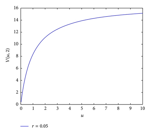
Example 1. Let c₁ = 0.1, c₂ = 0.2, μ = 5, α = β = π/4, λ = 3, b = 2, σ = 0.05, δ = 0.006, , , d = 1/4000, and r = 0.05, the result is shown in Figure 1.

From Figure 1, we see that V(u; 2) is an increasing function with respect to u.

Details are in the caption following the image — **Figure 1**
Open in figure viewer PowerPoint

The expected present value of total dividends V(u; 2).

Acknowledgments

This work was supported in part by the National Natural Science Foundation of China under Grant nos. 61370096 and 61173012 and the Key Project of Natural Science Foundation of Hunan Province under Grant no. 12JJA005.

Appendix

The sinc method is a highly efficient numerical method developed by Stenger, the pioneer of this field, people in his school, and others [18–22]. It is widely used in various fields of numerical analysis such as interpolation, quadrature, approximation of transforms, and solution of integral, ordinary differential, and partial differential equations.

sinc methods are based on the use of the cardinal function, C(f, h), which is sinc expansion of function f, defined by

(A.1)

where the step size h > 0, and the function sinc is defined on the whole real line, −∞ < x < ∞, by

(A.2)

For any h > 0, the translated sinc functions with evenly spaced nodes are given as

(A.3)

The sinc functions are cardinal for the interpolating points kh in the sense that

(A.4)

Definition A.1 (see [19], P73, De. 1.5.2.)Let ϕ denote a smooth one-to-one transformation of an arc Γ with end-point t₁ and t₂ onto ℝ, such that ϕ(t₁) = −∞ and ϕ(t₂) = ∞. Let ψ = ϕ⁻¹ denote the inverse map, so that

(A.5)

Given ϕ, ψ, and a positive number h, define the sinc points z_k by

(A.6)

and a function ρ by

(A.7)

Observe that ρ(z) increases from 0 to ∞ as z traverses Γ from t₁ to t₂.

Corresponding to positive numbers , , and d, let denote the family of all functions f defined on Γ for which

(A.8)

such that the Fourier transform {f∘ϕ⁻¹} ^~ satisfies the following relation:

(A.9)

for all ζ ∈ ℝ.

Another important family of functions is , with , and 0 < d < π. It consists of all those functions f defined on Γ such that and where Lf is defined by Lf = (f(t₁) + ρ(x)f(t₂))/(1 + ρ(x)).

Let N and M denote two positive integers, such that , or where [·] denotes the greatest integer function. Moreover, we denote m = M + N + 1.

Definition A.2. Given three positive integers N, M, and m as above, let D_m and V_m denote linear operators acting on functions f defined on Γ given by

(A.10)

where z_j = ψ(jh) denote the sinc points. Set

(A.11)

and we then define an m × m matrix I⁽⁻¹⁾ by

, with

denoting the (i, j)th element of I⁽⁻¹⁾. Finally, let ∥·∥ denote the uniform norm on Γ that is,

(A.12)

Theorem A.3 (see [19], P85, Th. 1.5.13.)Let ; then, as N → ∞,

(A.13)

, then it is convenient to take w_j = γ_j = S(j, h)∘ϕ, j = −M, …, N.

Theorem A.4 (see [19], P87, Th. 1.5.14.)Let ; then,

(A.14)

Theorem A.5 (see [19], P93, Th. 1.5.19.)Let ; then, for all N > 1,

(A.15)

where

(A.16)

with (I⁽⁻¹⁾) ^T denoting the transpose of I⁽⁻¹⁾.

Theorem A.6 (see [19], P95-96, Th. 1.5.20.)Let ; suppose that A^± can be diagonalized with A⁺ = XSX⁻¹ and with A⁻ = YSY⁻¹ and that S is a diagonal matrix. If for some positive c^′ independent of N, one has F^′(s) ≤ c^′ for all ℜs ≥ 0, then there exists a constant C independent of N such that

(A.17)

where

(A.18)

(A.19)

with c^′′ ≥ t₂ − t₁.

Theorem A.7 (see [18], P106, Th. 4.1.)Let ϕ be a conformal one-to-one transformation of an arc Γ. Then,

(A.20)

References

1 Avanzi B., Gerber H. U., and Shiu E. S. W., Optimal dividends in the dual model, Insurance: Mathematics and Economics. (2007) 41, no. 1, 111–123, https://doi.org/10.1016/j.insmatheco.2006.10.002, MR2324568, ZBL1131.91026.
10.1016/j.insmatheco.2006.10.002
Web of Science® Google Scholar
2 Avanzi B. and Gerber H. U., Optimal dividends in the dual model with diffusion, ASTIN Bulletin. (2008) 38, no. 2, 653–667, https://doi.org/10.2143/AST.38.2.2033357, MR2655288, ZBL05570365.
10.2143/AST.38.2.2033357
Web of Science® Google Scholar
3 Cramér H., Collective Risk Theory: A Survey of the Theory from the Point of View of the Theory of Stochastic Process, 1955, Ab Nordiska Bokhandeln, Stockholm, Sweden.
Google Scholar
4 Seal H. L., Stochastic Theory of a Risk Business, 1969, John Wiley & Sons, New York, NY, USA.
Google Scholar
5 Takács L., Combinatorial Methods in the Theory of Stochastic Processes, 1967, John Wiley & Sons, New York, NY, USA.
Google Scholar
6 Bayraktar E. and Egami M., Optimizing venture capital investment in a jump diffusion model, Mathematical Methods of Operations Research. (2008) 67, no. 1, 21–42, https://doi.org/10.1007/s00186-007-0181-x.
10.1007/s00186-007-0181-x
Web of Science® Google Scholar
7 Yang H. and Zhu J., Ruin probabilities of a dual Markov-modulated risk model, Communications in Statistics—Theory and Methods. (2008) 37, no. 20, 3298–3307, https://doi.org/10.1080/03610920802117080.
10.1080/03610920802117080
Web of Science® Google Scholar
8 de Finetti B., Su un′impostazione alternativa della teoria collectiva del rischio, 2, Transactions of the 15th International Congress of Actuaries, 1957, 433–443.
Google Scholar
9 Bühlmann H., Mathematical Methods in Risk Theory, 1970, Springer, New York, NY, USA.
Google Scholar
10 Gerber H. U., Games of economic survival with discrete- and continuous-income processes, Operational Research. (1972) 20, no. 1, 37–45, https://doi.org/10.1287/opre.20.1.37.
10.1287/opre.20.1.37
Google Scholar
11 Gerber H. U., An Introduction to Mathematical Risk Theory, 1979, 8, R.Iwin, Homewood, Ill, USA, S.S. Heubner Foundation Monograph Series, MR579350.
Google Scholar
12 Albrecher H., Badescu A., and Landriault D., On the dual risk model with tax payments, Insurance: Mathematics and Economics. (2008) 42, no. 3, 1086–1094, https://doi.org/10.1016/j.insmatheco.2008.02.001, MR2435378, ZBL1141.91481.
10.1016/j.insmatheco.2008.02.001
Web of Science® Google Scholar
13 Gerber H. U. and Landry B., On the discounted penalty at ruin in a jump-diffusion and the perpetual put option, Insurance: Mathematics and Economics. (1998) 22, no. 3, 263–276, https://doi.org/10.1016/S0167-6687(98)00014-6, MR1650304, ZBL0924.60075.
10.1016/S0167-6687(98)00014-6
Web of Science® Google Scholar
14 Ng A. C. Y., On a dual model with a dividend threshold, Insurance: Mathematics and Economics. (2009) 44, no. 2, 315–324, https://doi.org/10.1016/j.insmatheco.2008.11.011, MR2517896, ZBL1163.91441.
10.1016/j.insmatheco.2008.11.011
Web of Science® Google Scholar
15 Lin X. S. and Pavlova K. P., The compound Poisson risk model with a threshold dividend strategy, Insurance: Mathematics and Economics. (2006) 38, no. 1, 57–80, https://doi.org/10.1016/j.insmatheco.2005.08.001, MR2197303, ZBL1157.91383.
10.1016/j.insmatheco.2005.08.001
Web of Science® Google Scholar
16 Gao S. and Liu Z. M., The perturbed compound Poisson risk model with constant interest and a threshold dividend strategy, Journal of Computational and Applied Mathematics. (2010) 233, no. 9, 2181–2188, https://doi.org/10.1016/j.cam.2009.10.004, MR2577757, ZBL1222.91023.
10.1016/j.cam.2009.10.004
Web of Science® Google Scholar
17 Wan N., Dividend payments with a threshold strategy in the compound Poisson risk model perturbed by diffusion, Insurance: Mathematics and Economics. (2007) 40, no. 3, 509–523, https://doi.org/10.1016/j.insmatheco.2006.08.002, MR2311547, ZBL1183.91077.
10.1016/j.insmatheco.2006.08.002
Web of Science® Google Scholar
18 Lund J. and Bowers K. L., Sinc Methods for Quadrature and Differential Equations, 1992, SIAM, Philadelphia, Pa, USA, https://doi.org/10.1137/1.9781611971637, MR1171217.
10.1137/1.9781611971637
Google Scholar
19 Stenger F., Numerical Methods Based on Sinc and Analytic Functions, 1993, 20, Springer, New York, NY, USA, Springer Series in Computational Mathematics, https://doi.org/10.1007/978-1-4612-2706-9, MR1226236.
10.1007/978-1-4612-2706-9
Google Scholar
20 Stenger F., Summary of Sinc numerical methods, Journal of Computational and Applied Mathematics. (2000) 121, no. 1-2, 379–420, https://doi.org/10.1016/S0377-0427(00)00348-4, MR1780056, ZBL0964.65010.
10.1016/S0377-0427(00)00348-4
Web of Science® Google Scholar
21 Stenger F., Handbook of Sinc Numerical Methods, 2011, CRC & Taylor & Francis, Boca Raton, Fla, USA, MR2722054.
Google Scholar
22 Chen X. and Ou H., A compound Poisson risk model with proportional investment, Journal of Computational and Applied Mathematics. (2013) 242, 248–260, https://doi.org/10.1016/j.cam.2012.10.027, MR2997440, ZBL06127787.
10.1016/j.cam.2012.10.027
Web of Science® Google Scholar

Citing Literature

All articles

The Perturbed Dual Risk Model with Constant Interest and a Threshold Dividend Strategy

Abstract

1. Introduction

2. Integrodifferential Equations

2.1. Integrodifferential Equations for M(u, y; b)

2.2. Integrodifferential Equations for V(u, b)

3. Numerical Analysis

3.1. Numerical Solution of the Expected Present Value of Total Dividends V(u; b)

4. Numerical Example

Acknowledgments

Appendix

References

Citing Literature

Figures

References

Information

About Wiley Online Library

Help & Support

Opportunities

Connect with Wiley

The Perturbed Dual Risk Model with Constant Interest and a Threshold Dividend Strategy

Abstract

1. Introduction

2. Integrodifferential Equations

2.1. Integrodifferential Equations for M(u, y; b)

2.2. Integrodifferential Equations for V(u, b)

3. Numerical Analysis

3.1. Numerical Solution of the Expected Present Value of Total Dividends V(u; b)

4. Numerical Example

Acknowledgments

Appendix

References

Citing Literature

Figures

References

Related

Information