Volume 2013, Issue 1 912579

Research Article

Open Access

Effects of Dispersal for a Logistic Growth Population in Random Environments

Xiaoling Zou,

Xiaoling Zou

Department of Mathematics, Harbin Institute of Technology (Weihai), Weihai 264209, China hit.edu.cn

Search for more papers by this author

Dejun Fan,

Corresponding Author

Dejun Fan

[email protected]

Department of Mathematics, Harbin Institute of Technology (Weihai), Weihai 264209, China hit.edu.cn

Search for more papers by this author

Ke Wang,

Ke Wang

Department of Mathematics, Harbin Institute of Technology (Weihai), Weihai 264209, China hit.edu.cn

School of Mathematics and Statistics, Northeast Normal University, Changchun 130024, China nenu.edu.cn

Search for more papers by this author

Xiaoling Zou,

Xiaoling Zou

Department of Mathematics, Harbin Institute of Technology (Weihai), Weihai 264209, China hit.edu.cn

Search for more papers by this author

Dejun Fan,

Corresponding Author

Dejun Fan

[email protected]

Department of Mathematics, Harbin Institute of Technology (Weihai), Weihai 264209, China hit.edu.cn

Search for more papers by this author

Ke Wang,

Ke Wang

Department of Mathematics, Harbin Institute of Technology (Weihai), Weihai 264209, China hit.edu.cn

School of Mathematics and Statistics, Northeast Normal University, Changchun 130024, China nenu.edu.cn

Search for more papers by this author

First published: 21 March 2013

https://doi.org/10.1155/2013/912579

Citations: 5

Academic Editor: Julio Rossi

Share a link

Email
Wechat
Bluesky

Abstract

We study a stochastic logistic model with diffusion between two patches in this paper. Using the definition of stationary distribution, we discuss the effect of dispersal in detail. If the species are able to have nontrivial stationary distributions when the patches are isolated, then they continue to do so for small diffusion rates. In addition, we use some examples and numerical experiments to reflect that diffusions are capable of both stabilizing and destabilizing a given ecosystem.

1. Introduction

Dispersal is a ubiquitous phenomenon in the natural world. This phenomenon plays a very important role in understanding the ecological and evolutionary dynamics of populations. The theoretical studies of spatial distributions can be traced back as far as Skellam [1]. Then many scholars have focused on the effects of spatial factors which play a crucial role in the study of stability. Some mathematical models dealt with a single population dispersing among patches (see [2–9] and references cited therein). The others dealt with competition or predator-prey interactions in patchy environments (see [10–16] and references cited therein). These models centered round local and global stability of equilibrium points, persistence, and extinction of populations.

Through the studies for the diffusion systems and the corresponding ones without diffusion, many authors have discussed the relationship between the existence of the equilibriums and their stability. Levin [10] showed that two unstable competitive patches can be stabilized by diffusion; Levin [11] also showed that diffusion can destabilize a stable system by using a prey-predator model; Allen [4] proved that a single species diffusion system remains weakly persistent if the strength of diffusion is small enough; Beretta and Takeuchi [5, 6] showed that small diffusion cannot change the global stability of the model. Takeuchi also proved that diffusion among patches will not destabilize single-population dynamics [9].

However, the most natural phenomena do not follow strictly deterministic laws, but rather oscillate randomly about some averages. That is to say populations in the real word are inevitably affected by various environmental noises which is an important phenomenon in ecosystems [17–19]. So we will consider a stochastic diffusion system which is composed of two patches and connected by diffusion. Then we want to know ‘‘how are the effects of dispersal under random environments?” According to the author′s best knowledge, there are few results dealing with this problem, and stabilizing and/or destabilizing effects of dispersal remain largely unknown due to difficulties involved by random disturbances. Generally speaking, there does not have time independent equilibrium point for a stochastic system. Hence we will investigate the effects of dispersal by the concept of stationary distribution (some analogue which plays the role of the deterministic equilibrium point and reflects the stability to some extent). In this paper, we will show that diffusion cannot change the existence of stable stationary distribution for the stochastic model if the strength of diffusion is small enough. Moreover, small diffusion rates have some stabilizing effects, and large diffusion rates have some destabilizing effects on the stochastic model. That is, diffusions are capable of both stabilizing and destabilizing a given ecosystem.

2. Formulation of the Mathematical Model

The classical mathematical model describing the dynamics of a single species is the logistic model, governed by the following differential equation:

()

This is a very popular model, and many scholars have considered various ecosystems based on this equation. If we take the dispersal phenomenon into consideration, a single population dispersing in two patches becomes

()

where x_i represents the population density of the species in ith patch. r_i and k_i are the growth rate and self-competition coefficient of the population in the ith patch. ε_ij is a nonnegative diffusion coefficient for the species from jth patch to ith patch (i ≠ j). It is supposed that the net exchange from ith patch to jth patch is proportional to the difference of population densities x_i − x_j in each patch as the usual assumption (see [2, 4–6, 20, 21]).

Taking the effect of randomly fluctuating environment into consideration, we incorporate white noises in deterministic models. We assume that fluctuations in the environments will manifest themselves mainly as fluctuations in the growth rates of the populations. We usually estimate them by average values plus error terms which follow normal distributions in practice. Let

()

where B₁(t), B₂(t) are mutually independent Brownian motions and σ₁ and σ₂ reflect the intensities of the white noises. Then, the corresponding Itô-type stochastic system which takes the dispersal phenomenon into consideration becomes

()

Throughout this paper, unless otherwise specified, we let (Ω, F, {ℱ} _t≥0, P) be a complete probability space. {ℱ} _t≥0 is a filtration defined on this space satisfying the usual conditions (It is right continuous, and ℱ₀ contains all P-null sets.).

3. Existence and Uniqueness of the Positive Solution for System (4)

Population densities x₁(t) and x₂(t) should be nonnegative by their biological significance. For this reason, we want to study system (4) in the region

()

Now, we will show that

is a positive invariant set.

Theorem 1. For any initial value , there is a unique solution (x₁(t), x₂(t)) to system (4) on t ≥ 0, and the solution will remain in with probability 1.

Proof. Our proof is motivated by the works of Mao et al. [22]. All the coefficients in system (4) are locally Lipschitz continuous; then for any given initial value , there is a unique maximal local solution (x₁(t), x₂(t)) on t ∈ [0, τ_e], where τ_e is an explosion time (see e.g. [23, 24]). In order to show this solution is global, we only need to prove τ_e = ∞. Let k₀ > 0 be so large that x_i(0), i = 1,2 lying within the interval [1/k₀, k₀]. For each integer k > k₀, define stopping times as follows:

()

It is easy to see τ_k is increasing as k → ∞. Set τ_∞ = lim_k→∞τ_k; hence τ_∞ ≤ τ_e a.s. If we can prove τ_∞ = ∞ a.s., then τ_e = ∞ a.s. and

a.s. for all t ≥ 0. In other words, we only need to prove τ_∞ = ∞ a.s.. For if this statement is false, then there are two constants T > 0 and ε ∈ (0,1) such that

()

Consequently, there is an integer k₁ ≥ k₀ satisfying

()

for all k ≥ k₁. Define a C²-function

()

The nonnegativity of this function can be seen from

()

, Itô′s formula shows that

()

There exists a constant N such that f(x) = x^−0.5 − x⁻¹ < N on t > 0; so we can obtain

()

as long as

. Integrating both sides from 0 to τ_k ∧ T and then taking expectations yield

()

Denote Ω_k = {τ_k ≤ T} for k ≥ k₁, by (8), P(Ω_k) ≥ ε. Note that, for every ω ∈ Ω_k, there is some i such that x_i(τ_k, ω) equals either k or 1/k, and V(x₁(τ_k, ω), x₂(τ_k, ω)) is no less than either

. Consequently,

()

It is follows from (13) that

()

Letting k → ∞ leads to the contradiction

()

So we must have τ_∞ = ∞ a.s.

Theorem 1 shows that the solution of system (4) will remain in the positive cone . This nice positive invariant property provides us with a great opportunity to construct different types of the Lyapunov functions to discuss the stationary distribution for system (4) in in more detail.

4. Stationary Distribution for System (4)

In order to prove our main results, we require some results in [25], and the technique we used here is motivated by [26–28]. System (4) can be rewritten as

()

Its diffusion matrix can be presented as

()

Assumption B. There exists a bounded domain with regular boundary, having the following properties.

(B1)
In the domain U and some neighborhood thereof, the smallest eigenvalue of the diffusion matrix A(x) is bounded away from zero.
(B2)
for all n, where K_n is a family of countable compact subsets such that ; E_xτ is the mean time τ at which a path issuing from x reaches the set K_n.

Lemma 2 (see [25].)If (B) holds, then the Markov process X(t) = (x₁, x₂) has a stable stationary distribution μ(·) confined on .

To validate (B1), it suffices to prove F is uniformly elliptical in U, where Fu = b(x) · u_x + [tr(A(x)u_xx)]/2; that is, there is a positive number M such that

()

(see Chapter 3 of [29] and Rayleigh′s principle in [30]). To verify (B2), it suffices to show that there exists some neighborhood U and a nonnegative C²-function such that, for any x ∈ E_l ∖ U, LV is negative (see[31]).

The deterministic system (2) has two equilibrium points, namely, E₀(0,0) and . Takeuchi [9] has proved that this single species diffusion model has a positive and globally stable equilibrium point for any diffusion rate; the results obtained in his paper show that no diffusion rate; can change the global stability of the deterministic model.

Suppose

is the equilibrium points of system (2). Then, they meet the following equations:

()

These relations will be useful in the proof of the next theorem. Next, we will show the conditions under which system (4) exists on a stable stationary distribution and discuss the effect of diffusion on the stochastic system.

Theorem 3. Let σ₁ > 0, σ₂ > 0 such that

()

Then there is a stationary distribution μ(·) with respect to

for system (4) with any initial value

, where

()

In addition, condition (22) can be satisfied when

()

Proof. Define ,

()

where k is a positive constant to be determined later. V(x₁, x₂) is a positive definite function for all

. By Itô′s formula, we can calculate

()

Then we have

()

Choosing k = ε₁₂/ε₂₁, we can obtain

()

where

()

Then we have

()

If we denote

, then

()

It is well known that

is an elliptic-curve when

()

that is,

()

Now we take U to be the intersection of (

) and

with

. So, for

, LV is negative, which implies condition (B2) is satisfied. Besides, If U is bounded away from (0,0), that is,

()

which can be satisfied when

()

then there is a constant M > 0 such that

()

which implies condition (B1) is also satisfied. Therefore, system (4) has a stable stationary distribution μ(·) confined on

. These together with the positive invariant property of

complete our proof.

Lemma 4 (see [32], Corollary 1.)Equation dx(t) = x(t)(r − kx(t))dt + αx(t)dB(t) has a nontrivial stationary distribution if and only if α² < 2r.

Remark 5. Suppose there is no diffusion; that is, ε₁₂ = ε₂₁ = 0. Then condition (21) is always satisfied, and the corresponding equations,

()

have stationary distributions when

. This is in agreement with the results in the literature [32] (see Lemma 4).

Remark 6. Suppose condition (24) is satisfied. Then the species has a nontrivial stationary distribution in all patches if the patches are isolated; that is, the diffusion among patches is neglected, and the species is confined to each patch. Condition (21) can be satisfied when we choose ε₁₂, ε₂₁ sufficiently small. Then we have a conclusion that diffusion cannot change the existence of stable stationary distribution for stochastic system if the strength of diffusion rate is small enough.

Remark 7. An immediate consequence of condition (22) is that environmental noises are against the stationary distribution for stochastic system. If , ; that is, only species in the 2nd patch have a nontrivial stationary distribution when there is no diffusion. But we can choose ε₂₁ sufficiently small such that conditions in Theorem 3 are satisfied, and there exists a stationary distribution for (x₁(t), x₂(t)). This implies small diffusion rate has some stabilizing effects on stochastic system. However, if we choose ε₂₁ sufficiently large, then the conditions of Theorem 3 are destroyed which implies large diffusion rate also has some destabilizing effects on stochastic models.

5. Examples and Numerical Simulation

Now we will give three examples to explain both the stabilizing and destabilizing effects of diffusion on the population dynamics. The data we used here are only some hypothetical data which are used to explain the effect of diffusion. We use the Milsteins Higher Order Method mentioned in [33] to numerically simulate (4):

()

where ξ_k and η_k are the Gaussian random variables N(0,1).

It is very difficult to choose parameters in the system from realistic estimation. The estimation of the parameters can be derived by some statistical methods and filtering theory which are linked to statistical problems and filtering problems. Therefore, we will only use some hypothetical parameters to verify the theoretical effects in this section.

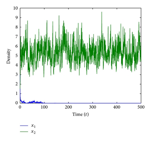
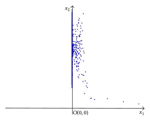
Example 8. For system (38), we let r₁ = 0.9, k₁ = 1.2, , r₂ = 1.1, k₂ = 0.2, and σ₂ = 0.8. Note that and ; so for system (38), species in the 1st patch has a Dirac delta distribution with mass concentrated in 0, and species in the 2nd patch has a nontrivial distribution. (see literature [32].) Numerical simulations of (38) are showed in Figures 1(a) and 1(b).

Details are in the caption following the image — **Figure 1 (a)**
Open in figure viewer PowerPoint

Numerical simulations of Example 8 (there is no diffusion). Species in the 1st patch has a Dirac delta distribution with mass concentrated in 0, and species in the 2nd patch has a stationary distribution.

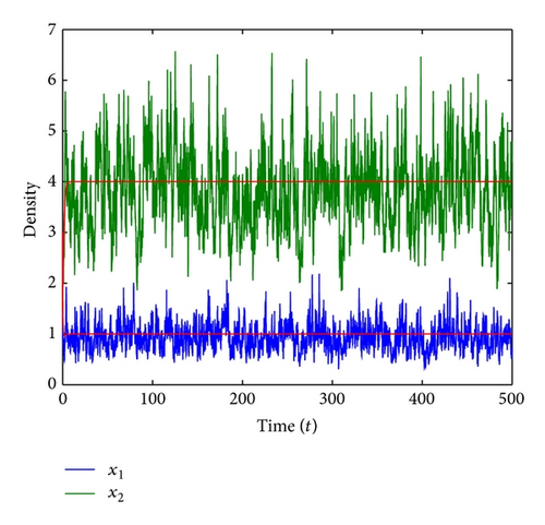
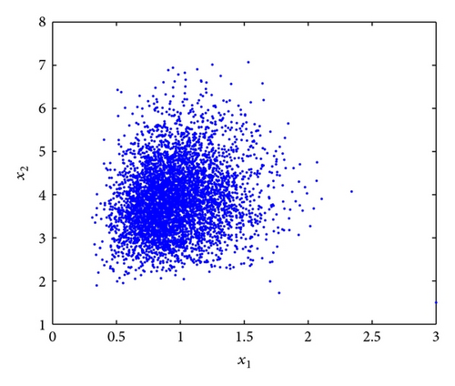
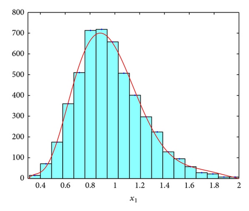
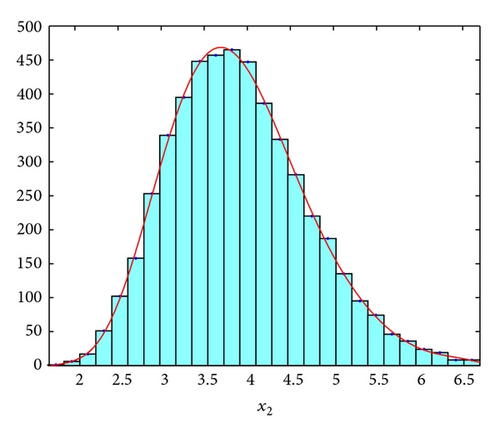
Example 9. For system (4), we let r₁ = 0.9, k₁ = 1.2, ε₁₂ = 0.1, , r₂ = 1.1, k₂ = 0.2, ε₂₁ = 0.4, and σ₂ = 0.8. Its corresponding deterministic system (2) has a globally asymptotically stable equilibrium point E^*(x^*, y^*) = (1,4). We also have

()

So, from Theorem 3, we obtain that there is a stationary distribution μ(·) with respect to

for system (4) with initial value

(see Figures 2(a), 2(b), 2(c), and 2(d)). The stabilizing effect of small diffusion rate can be seen clearly from this example.

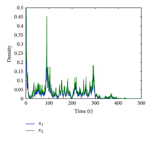
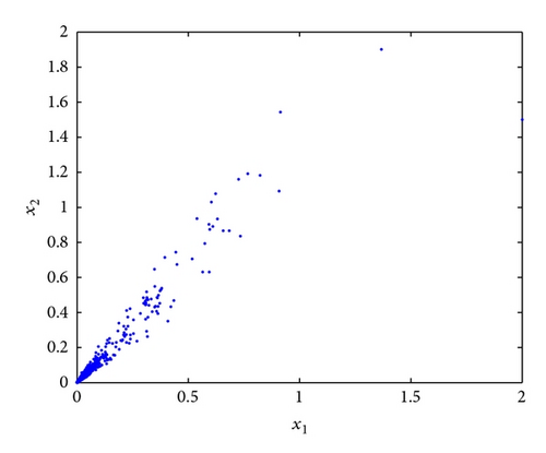
Example 10. For system (4), we let r₁ = 0.9, k₁ = 1.2, ε₁₂ = 0.1, , r₂ = 1.1, k₂ = 0.2, ε₂₁ = 5, and σ₂ = 0.8. It is clear that conditions of Theorem 3 are destroyed and numerical simulations of this example showed in Figures 3(a) and 3(b). The destabilizing effect of large diffusion rate can be seen clearly from this example.

6. Concluding Remarks

The main objective of this paper is to study the effects of dispersal on stationary distribution for a stochastic logistic diffusion system. We show that the dispersal stabilizes the system when the dispersal rate is small, and destabilizes the system, when the dispersal rate is large. Our results show that small dispersal rate cannot change the existence of stationary distribution for the stochastic model such as it cannot change the global stability of the deterministic model. Though diffusions have stabilizing effects, our examples show that dispersal may also have the side effects which result in destabilization. This suggests that dispersal among patches should be regulated. Their ecological implications are that neither no diffusion nor unlimited diffusion may serve the interest of stabilizing the given ecosystem in random environments! This observation may be useful in planning and controlling of ecosystems.

Acknowledgments

The authors would like to thank the editor and the referees for their suggestions which improved the presentation of this paper. This paper was partially supported by Grants from the National Natural Science Foundation of China (no. 11171081), (no. 11171056), (no. 11126219), (no. 11001032), and (no. 11101183), Shandong Provincial Natural Science Foundation of China (Grant no. ZR2011AM004), and Natural Scientific Research Innovation Foundation in Harbin Institute of Technology (HIT.NSRIF.2011094).

References

1 Skellam J. G., Random dispersal in theoretical populations, Biometrika. (1951) 38, 196–218, MR0043440, ZBL0043.14401.
10.1093/biomet/38.1-2.196
CAS PubMed Web of Science® Google Scholar
2 Hastings A., Dynamics of a single species in a spatially varying environment: the stabilizing role of high dispersal rates, Journal of Mathematical Biology. (1982) 16, no. 1, 49–55, https://doi.org/10.1007/BF00275160, MR693372.
10.1007/BF00275160
Web of Science® Google Scholar
3 Freedman H. I., Rai B., and Waltman P., Mathematical models of population interactions with dispersal. II. Differential survival in a change of habitat, Journal of Mathematical Analysis and Applications. (1986) 115, no. 1, 140–154, https://doi.org/10.1016/0022-247X(86)90029-6, MR835590, ZBL0588.92020.
10.1016/0022-247X(86)90029-6
Web of Science® Google Scholar
4 Allen L. J. S., Persistence, extinction, and critical patch number for island populations, Journal of Mathematical Biology. (1987) 24, no. 6, 617–625, https://doi.org/10.1007/BF00275506, MR880448, ZBL0603.92019.
10.1007/BF00275506
CAS PubMed Web of Science® Google Scholar
5 Beretta E. and Takeuchi Y., Global stability of single-species diffusion Volterra models with continuous time delays, Bulletin of Mathematical Biology. (1987) 49, no. 4, 431–448, https://doi.org/10.1016/S0092-8240(87)80005-8, MR908159, ZBL0627.92021.
10.1007/BF02458861
CAS PubMed Web of Science® Google Scholar
6 Beretta E. and Takeuchi Y., Global asymptotic stability of Lotka-Volterra diffusion models with continuous time delay, SIAM Journal on Applied Mathematics. (1988) 48, no. 3, 627–651, https://doi.org/10.1137/0148035, MR941104, ZBL0661.92018.
10.1137/0148035
Web of Science® Google Scholar
7 Wang W. and Chen L., Global stability of a population dispersal in a two-patch environment, Dynamic Systems and Applications. (1997) 6, no. 2, 207–215, MR1461438, ZBL0892.92026.
Google Scholar
8 Cui J., Takeuchi Y., and Lin Z., Permanence and extinction for dispersal population systems, Journal of Mathematical Analysis and Applications. (2004) 298, no. 1, 73–93, https://doi.org/10.1016/j.jmaa.2004.02.059, MR2085492, ZBL1073.34052.
10.1016/j.jmaa.2004.02.059
Web of Science® Google Scholar
9 Takeuchi Y., Cooperative systems theory and global stability of diffusion models, Acta Applicandae Mathematicae. (1989) 14, no. 1-2, 49–57, https://doi.org/10.1007/BF00046673, MR990035, ZBL0665.92017.
10.1007/BF00046673
Web of Science® Google Scholar
10 Levin S. A., Dispersion and population interactions, The American Naturalist. (1974) 108, no. 960, 207–228, https://doi.org/10.1086/282900.
10.1086/282900
Web of Science® Google Scholar
11 Levin S. A., Spatial patterning and the structure of ecological communities, Some Mathematical Questions in Biology, 1976, 8, American Mathematical Society, Providence, RI, USA, 1–35, Lectures on Mathematics in the Life Sciences, MR0465284, ZBL0338.92017.
Google Scholar
12 Freedman H. I. and Takeuchi Y., Global stability and predator dynamics in a model of prey dispersal in a patchy environment, Nonlinear Analysis. Theory, Methods & Applications. (1989) 13, no. 8, 993–1002, https://doi.org/10.1016/0362-546X(89)90026-6, MR1009083, ZBL0685.92018.
10.1016/0362-546X(89)90026-6
Web of Science® Google Scholar
13 Kuang Y. and Takeuchi Y., Predator-prey dynamics in models of prey dispersal in two-patch environments, Mathematical Biosciences. (1994) 120, no. 1, 77–98, https://doi.org/10.1016/0025-5564(94)90038-8, MR1281745, ZBL0793.92014.
10.1016/0025-5564(94)90038-8
CAS PubMed Web of Science® Google Scholar
14 Takeuchi Y., Diffusion-mediated persistence in two-species competition Lotka-Volterra model, Mathematical Biosciences. (1989) 95, no. 1, 65–83, https://doi.org/10.1016/0025-5564(89)90052-7, MR1001292, ZBL0671.92022.
10.1016/0025-5564(89)90052-7
CAS PubMed Web of Science® Google Scholar
15 Li J. and Yan J., Permanence and extinction for a nonlinear diffusive predator-prey system, Nonlinear Analysis. Theory, Methods & Applications. (2009) 71, no. 1-2, 399–417, https://doi.org/10.1016/j.na.2008.10.087, MR2518047, ZBL1173.34033.
10.1016/j.na.2008.10.087
Web of Science® Google Scholar
16 Takeuchi Y. and Lu Z. Y., Permanence and global stability for competitive Lotka-Volterra diffusion systems, Nonlinear Analysis. Theory, Methods & Applications. (1995) 24, no. 1, 91–104, https://doi.org/10.1016/0362-546X(94)E0024-B, MR1308472, ZBL0823.34056.
10.1016/0362-546X(94)E0024-B
Web of Science® Google Scholar
17 Gard T. C., Persistence in stochastic food web models, Bulletin of Mathematical Biology. (1984) 46, no. 3, 357–370, https://doi.org/10.1016/S0092-8240(84)80044-0, MR748544, ZBL0533.92028.
10.1016/S0092-8240(84)80044-0
Web of Science® Google Scholar
18 Gard T. C., Stability for multispecies population models in random environments, Nonlinear Analysis. Theory, Methods & Applications. (1986) 10, no. 12, 1411–1419, https://doi.org/10.1016/0362-546X(86)90111-2, MR869549, ZBL0598.92017.
10.1016/0362-546X(86)90111-2
Web of Science® Google Scholar
19 May R. M., Stability and Complexity in Model Ecosystems, 1973, Princeton University, Princeton, NJ, USA.
10.1046/j.1365-2656.2000.00396.x
Google Scholar
20 Fan M. and Wang K., Study on harvested population with diffusional migration, Journal of Systems Science and Complexity. (2001) 14, no. 2, 139–148, MR1840921, ZBL0976.92023.
Google Scholar
21 Zou X. and Wang K., The protection zone of biological population, Nonlinear Analysis. Real World Applications. (2011) 12, no. 2, 956–964, https://doi.org/10.1016/j.nonrwa.2010.08.019, MR2736184, ZBL1203.92069.
10.1016/j.nonrwa.2010.08.019
Web of Science® Google Scholar
22 Mao X., Marion G., and Renshaw E., Environmental Brownian noise suppresses explosions in population dynamics, Stochastic Processes and Their Applications. (2002) 97, no. 1, 95–110, https://doi.org/10.1016/S0304-4149(01)00126-0, MR1870962, ZBL1058.60046.
10.1016/S0304-4149(01)00126-0
Web of Science® Google Scholar
23 Arnold L., Stochastic Differential Equations: Theory and Applications, 1972, John Wiley & Sons, New York, NY, USA.
Google Scholar
24 Friedman A., Stochastic Differential Equations and Applications. Vol. 2. Probability and Mathematical Statistics, 1976, 28, Academic Press, New York, NY, USA, MR0494491.
Google Scholar
25 Hasminskiĭ R. Z., Stochastic Stability of Differential Equations, 1980, 7, Sijthoff & Noordhoff, Alphen aan den Rijn, The Netherlands, Monographs and Textbooks on Mechanics of Solids and Fluids: Mechanics and Analysis, MR600653.
10.1007/978-94-009-9121-7
Google Scholar
26 Ji C., Jiang D., and Shi N., A note on a predator-prey model with modified Leslie-Gower and Holling-type II schemes with stochastic perturbation, Journal of Mathematical Analysis and Applications. (2011) 377, no. 1, 435–440, https://doi.org/10.1016/j.jmaa.2010.11.008, MR2754843, ZBL1216.34040.
10.1016/j.jmaa.2010.11.008
Web of Science® Google Scholar
27 Ji C. and Jiang D., Dynamics of a stochastic density dependent predator-prey system with Beddington-DeAngelis functional response, Journal of Mathematical Analysis and Applications. (2011) 381, no. 1, 441–453, https://doi.org/10.1016/j.jmaa.2011.02.037, MR2796222, ZBL1232.34072.
10.1016/j.jmaa.2011.02.037
Web of Science® Google Scholar
28 Mao X., Stationary distribution of stochastic population systems, Systems & Control Letters. (2011) 60, no. 6, 398–405, https://doi.org/10.1016/j.sysconle.2011.02.013, MR2841483.
10.1016/j.sysconle.2011.02.013
Web of Science® Google Scholar
29 Gard T. C., Introduction to Stochastic Differential Equations, 1988, 270, Madison Avenue, New York, NY, USA.
Google Scholar
30 Strang G., Linear Algebra and Its Applications, 1988, 3rd edition, Harcourt Brace, Watkins, Minn, USA.
Google Scholar
31 Zhu C. and Yin G., Asymptotic properties of hybrid diffusion systems, SIAM Journal on Control and Optimization. (2007) 46, no. 4, 1155–1179, https://doi.org/10.1137/060649343, MR2346378, ZBL1140.93045.
10.1137/060649343
Web of Science® Google Scholar
32 Pasquali S., The stochastic logistic equation: stationary solutions and their stability, Rendiconti del Seminario Matematico della Università di Padova. (2001) 106, 165–183, MR1876219, ZBL1165.60328.
Google Scholar
33 Higham D. J., An algorithmic introduction to numerical simulation of stochastic differential equations, SIAM Review. (2001) 43, no. 3, 525–546, https://doi.org/10.1137/S0036144500378302, MR1872387, ZBL0979.65007.
10.1137/S0036144500378302
Web of Science® Google Scholar

All articles

Effects of Dispersal for a Logistic Growth Population in Random Environments

Abstract

1. Introduction

2. Formulation of the Mathematical Model

3. Existence and Uniqueness of the Positive Solution for System (4)

4. Stationary Distribution for System (4)

5. Examples and Numerical Simulation

6. Concluding Remarks

Acknowledgments

References

Figures

References

Information

About Wiley Online Library

Help & Support

Opportunities

Connect with Wiley

Effects of Dispersal for a Logistic Growth Population in Random Environments

Abstract

1. Introduction

2. Formulation of the Mathematical Model

3. Existence and Uniqueness of the Positive Solution for System (4)

4. Stationary Distribution for System (4)

5. Examples and Numerical Simulation

6. Concluding Remarks

Acknowledgments

References

Figures

References

Related

Information