Volume 2013, Issue 1 912373

Research Article

Open Access

A Convex Adaptive Total Variation Model Based on the Gray Level Indicator for Multiplicative Noise Removal

Gang Dong,

Gang Dong

Department of Mathematics, Harbin Institute of Technology, Harbin 150001, China hit.edu.cn

Search for more papers by this author

Zhichang Guo,

Corresponding Author

Zhichang Guo

[email protected]

Department of Mathematics, Harbin Institute of Technology, Harbin 150001, China hit.edu.cn

Search for more papers by this author

Boying Wu,

Boying Wu

Department of Mathematics, Harbin Institute of Technology, Harbin 150001, China hit.edu.cn

Search for more papers by this author

Gang Dong,

Gang Dong

Department of Mathematics, Harbin Institute of Technology, Harbin 150001, China hit.edu.cn

Search for more papers by this author

Zhichang Guo,

Corresponding Author

Zhichang Guo

[email protected]

Department of Mathematics, Harbin Institute of Technology, Harbin 150001, China hit.edu.cn

Search for more papers by this author

Boying Wu,

Boying Wu

Department of Mathematics, Harbin Institute of Technology, Harbin 150001, China hit.edu.cn

Search for more papers by this author

First published: 06 June 2013

https://doi.org/10.1155/2013/912373

Citations: 9

Academic Editor: Guoyin Li

Share a link

Email
Wechat
Bluesky

Abstract

This paper focuses on the problem of multiplicative noise removal. Using a gray level indicator, we derive a new functional which consists of the adaptive total variation term and the global convex fidelity term. We prove the existence, uniqueness, and comparison principle of the minimizer for the variational problem. The existence, uniqueness, and long-time behavior of the associated evolution equation are established. Finally, experimental results illustrate the effectiveness of the model in multiplicative noise reduction. Different from the other methods, the parameters in the proposed algorithms are found dynamically.

1. Introduction

Multiplicative noise occurs while one deals with active imaging system, such as laser images, microscope images, and SAR images. Given a noisy image f : Ω → R, where Ω is a bounded open subset of ℝ², we assume

()

where u is the true image and η is the noise. In what follows we will always assume that f > 0 and u > 0. Some prior information about the mean and variance of the multiplicative noise is as follows:

()

where |Ω | = ∫_Ω 1 dx. Our purpose is to remove noise in images while preserving the maximum information about u.

The goal of this paper is to propose a globally strictly convex functional well-adapted to removing multiplicative noise, which is as follows:

()

where f is noisy image and

stands for the adaptive total variation of u. In the new model, we introduce a control factor, α(x), which controls the speed of diffusion at different region: at the low gray level (α(x) → 0), the speed is slow; at the high gray level (α(x) → 1), the speed is fast. The second term in the functional, that is, the fidelity term is global convex, which implies the constraint (2).

Various adaptive filters for multiplicative noise removal have been proposed. In the beginning, variational methods for multiplicative noise reduction deal with the Gaussian multiplicative noise [1]. In actual life, the speckle noise [2] is more widespread, such as synthetic aperture radar (SAR) imagery [3, 4]. Then, Aubert and Aujol [5] propose a new variational method for Gamma multiplicative noise reduction. By the logarithm transform, a large variety of methods rely on the conversion of the multiplicative noise into additive noise.

1.1. Gaussian Noise

In the additive noise case, the most classical assumption is that the noise is a white Gaussian noise. So one case in which dealing with multiplicative noise is the white Gaussian noise. Using the framework in [6], Rudin et al. [1] consider the following optimization problem for Gaussian multiplicative noise reduction:

()

where J(u) = ∫_Ω | ∇u| stands for the total variation of u, and H(u, f) is a fidelity term which consists of two integrals with two Lagrange multipliers:

()

In order to make sure the two constraints (2) and (3) are always satisfied during the evolution, by the gradient projection method, the authors evolve the following evolution equation:

()

If by the gradient projection method the values of λ₁ and λ₂ are found dynamically, the method is not always convex; while if λ₁, λ₂ > 0 are fixed, the corresponding minimization problem will lead to a sequence of constant function u approaching +∞.

1.2. Gamma Noise

Generally, the speckle noise is treated as Gamma noise with mean equal to one. The probability distribution function g(η) of the noise η takes the following form:

()

Gamma noise is more complex than Gaussian noise [2]. Based on maximum a posteriori (MAP) on p(u∣f), Aubert and Aujol [5] assume that the noise η follows a Gamma probability distribution with mean equal to one and p(u) following a Gibbs prior and then derive a functional formulating the following minimization problem (called AA model):

()

where S(Ω) = {u > 0, u ∈ BV(Ω)}. The new fidelity term H(u, f) = ∫_Ω (log u + (f/u))dx is strictly convex for u ∈ (0,2f). The authors prove the existence of a minimizer u ∈ S(Ω) to the minimization problem and derive existence and uniqueness results of the solution to the associated evolution equation:

()

1.3. The Model Based on the Logarithm Transform

The simplest idea is to take the log of both sides of (1),

()

which essentially converts the multiplicative problem into an additive one. If the distribution of the noise η takes the form (8), the expectation and the variance of the log-noise n are

()

where

()

is the polygamma function [7]. In [8], Shi and Osher use relaxed inverse scale space (RISS) flows to deal with various noises and provide iterative TV regularization. First, using the log-data log f, they propose the following model:

()

where w = log u. The corresponding RISS flow reads

()

with v(0) = 0, w(0) = c₀, for c₀ = ∫_Ω log fdx/|Ω|. Then, they generalize several multiplicative noise models [5, 9, 10], and for convergence reasons, use iterative TV regularization on exp (w) to obtain the RISS flow. And they investigate the properties of the flow and study the dependence on flow parameters.

1.4. The Model Based on the Exponent Transform

Recently, Huang et al. [11] utilize an exponential transformation u → e^u in the fidelity term of AA model to propose the following denoising model:

()

where α₁ > 0 and α₂ > 0 are regularization parameters, and w is an auxiliary variable. Next, they further develop an alternating minimization algorithm for the model (16) by incorporating another way of modified TV regularization in [12]. However, the mathematical analysis to the variational problem (16) is not given in [11]. By the exponential transformation u → e^u, Jin and Yang [13] change the fidelity term log u + fu of AA model (2) into u + fe^u and then study the following denoising model:

()

Notice that the fidelity term H(u, f) = ∫_Ω (u + fe^−u)dx is globally strictly convex. Based on this, they prove the uniqueness of the solutions to the variational problem (17) and show the existence and uniqueness of the weak solution for the following evolution equation corresponding to (17):

()

The paper is organized as follows. In Section 2, inspired from [1, 5, 14], based on the gray level indicator α(x), we derive a convex adaptive total variation model (4) for multiplicative noise removal. In Section 3, we prove the existence and uniqueness of the solution of the minimization problem (4). In Section 4, we study the associated evolution problem to the minimization problem (4). Specifically, we define the weak solution of the evolution problem, derive estimates for the solution of an approximating problem, prove existence and uniqueness of the weak solution, and discuss the behavior of the weak solution as t → ∞. In Section 5, we provide two numerical algorithms and experimental results to illustrate the effectiveness of our algorithms in image denoising. We also compare new algorithms with other ones.

2. A New Variational Model for Multiplicative Noise Removal

The goal of this section is to propose a new variational model for multiplicative noise removal. First, we proposed a new fidelity with global convexity, which can always satisfy the constraint (2) during the evolution. Then, by analyzing the properties of the noise, we propose the adaptive total variation based on a gray level indicator α(x).

2.1. A Global Convex Fidelity Term

Based on the idea in [15], we can obtain the following fidelity:

()

Note that H^′(u, f) = 1 − (f/u). Let us consider the following Euler-Lagrange equation for some functional-based problem:

()

where ∇u and ∇²u stand, respectively, for the gradient and the Hessian matrix of u with respect to the space variable x, and ℱ(∇u, ∇²u) is divergence operator from the functional. By integrating (20) in space, using integration by parts and the boundary condition (21) in the sense of distributions, we have

()

which implies the constraint (2). Moreover, using the idea in [6], the parameter λ can be calculated as

()

Remark 1. (1) It is easy to check that the function u → u + flog (1/u) reaches its minimum value f + flog (1/f) over ℝ⁺ for u = f.

(2) Let us denote by

()

We have h^′(u) = 1 − (f/u) = (u − f)/u, and h^′(u) = (f/u²) > 0, which deduce that the new fidelity term H(u, f) is globally strictly convex.

2.2. The Adaptive Total Variation Model

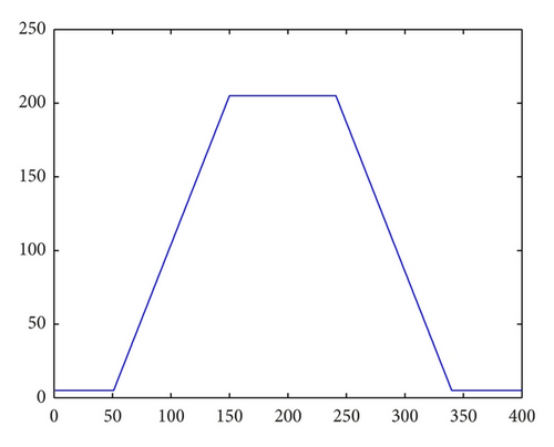
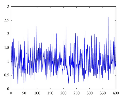
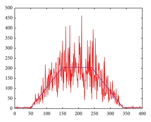
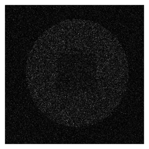
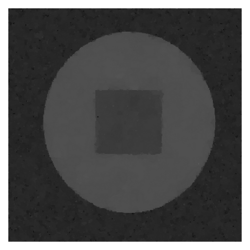
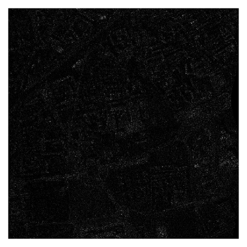
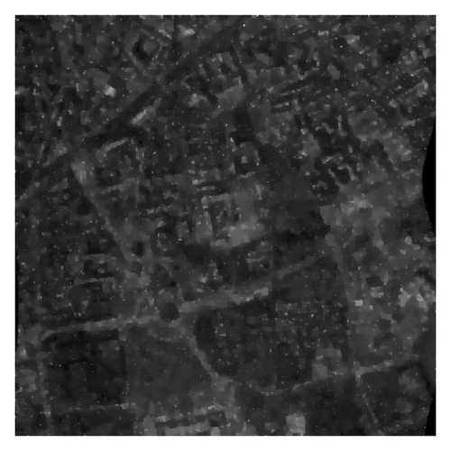
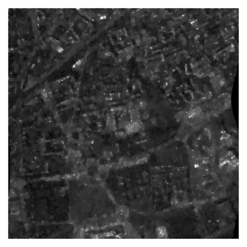
Assume u is a piecewise function, that is, , where Ω_i ∩ Ω_j = ∅, for i ≠ j, , and g_i is the gray level. Moreover, we assume that the samples of the noise on each pixel x are mutually independent and identically distributed (i.i.d.) with the probability density function η(x). For x ∈ Ω, f(x) = g_iη(x), and therefore, , where Var [f] and Var [η] are the variance of the noise image f and the noise at the pixel x, respectively. It is noticed that the variance of the noise is the constant σ² on each pixel, but the variance of the noise image f is influenced by the gray level. The higher the gray level is, the more remarkable the influence of the noise is. Especially, f = u when u = 0, and therefore f is noise free in this case. The fact is illustrious in Figure 1. It can be seen that in despite of the independent identically distribution of noise (see Figure 1(b)), the noise image shows different features on the pixel, where the gray levels are different (see Figure 1(d)).

Details are in the caption following the image — **Figure 1 (a) Noise-free signal**
Open in figure viewer PowerPoint

The relation between the influence of the noise and the gray levels. (a) 1D signal f; (b) 1D speckled noise with mean equal to 1 and L = 5; (c) f degraded by the speckled noise; (d) the compare between f and the noise signal f.

In [14], Chan and Strong propose the following adaptive total variation model:

()

where the weight function g(x) controls the speed of diffusion at different region. Utilizing this idea, we proposed a gray level indicator α(x). The indicator α(x) has such properties as follows: α(s) is monotonically increasing, g(0) = 0, α(s) ≥ 0, and α(s) → 1, as s → sup _x∈Ω u. Therefore, we propose the following gray indicators α(x):

()

where M = sup _x∈Ω (G_σ*f)(x), G_σ(x) = (1/4πσ)exp {−|x|²/4σ²}, σ > 0, and k > 0 are parameters. With this choice, α(x) is a positive-valued continuous function; α(x) is much smaller value at low gray levels (α(x) → 0) than at high gray levels (α(x) → 1) so that some small features at low gray levels are much less smoothed and therefore are preserved. As previously stated, at high gray levels, the region of the noise image is degraded more, while the region at low gray levels is degraded less (see Figure 1(d)). Then, from (26)/(27), at the high gray levels, α(x) → 1, the new model is more smooth at the region; at low gray levels, α(x) → 0, the new model is less smooth at the region.

The previous analysis leads us to propose a convex adaptive total variation model for multiplicative noise removal,

()

The evolution of the Euler-Lagrange equation for (28) is as follows:

()

3. The Minimization Problem (28)

In this section, we study the existence and uniqueness of the solution to the minimization problem (28), and then we consider the comparison principle for the problem (28).

3.1. Preliminaries

If f ∈ L^∞(Ω) with 0 < inf _x∈Ω f ≤ f ≤ sup _x∈Ω f, then

()

We always assume that Ω is a bounded open subset of ℝⁿ with Lipschitz boundary. As in [16], we introduce the following definition of α-total variation.

Definition 2. A function u ∈ L¹(Ω) has bounded α-total variation in Ω, if

()

where

()

Remark 3 (see [16].)(1) If u ∈ L¹(Ω) has bounded α-total variation in Ω, there is a Radon vector measure Du on Ω such that

()

(2) From (32), u ∈ L¹(Ω) having bounded α-total variation in Ω implies that u ∈ BV(Ω).

Now, we directly show some lemmas on α-total variation from [16].

Lemma 4. Assume that and u_k → u in L¹(Ω). Then, u ∈ BV(Ω), and

()

Lemma 5. Assume that u ∈ BV(Ω). Then, there exists a sequence such that

()

By a minor modification of the proof of Lemma 1 in Section 4.3 of [17], we can have the following lemma.

Lemma 6. Let u ∈ BV(Ω), and let φ_a,b be the cut-off function defined by

()

Then, Dφ_a,b(u) ∈ BV(Ω), and

()

3.2. Existence and Uniqueness of the Problem (28)

In this subsection, we show that problem (28) has at least one solution in BV(Ω).

Theorem 7. Let f ∈ L^∞(Ω) with inf _x∈Ω f > 0. Then, the problem (28) admits a unique solution u ∈ BV(Ω) such that

()

Proof. Let us rewrite

()

From Remark 1(1), we have

()

for u ∈ BV(Ω) with u > 0. This implies that E(u) has a lower bound for all u ∈ BV(Ω) with u > 0. Hence, there exists a minimizing sequence {u_n} ⊂ BV(Ω) for the problem (28).

Step 1. Let us denote a = inf _x∈Ω f and b = sup _x∈Ω f. We first claim that 0 < a ≤ u_n ≤ b.

In fact, we remark that h(s) is decreasing for s ∈ (0, f) and increasing for s ∈ (f, +∞). Therefore, if M ≥ f, one always has

()

Hence, if M = b = sup _x∈Ω f, we have

()

Moreover, utilizing Lemma 6, we can have

()

Combining (44) and (45), we deduce that

()

On the other hand, in the same way, we get that E(sup (u, a)) ≤ E(u). Therefore, we can assume that a ≤ u_n ≤ b without restriction.

Step 2. Let us prove that there exists u ∈ BV(Ω) such that

()

The proof in the Step 1 implies in particular that u_n is bounded in L¹(Ω). Since a ≤ u_n ≤ b and h(s) ∈ C[a, b], h(u_n) is bounded. Moreover, by the definition of {u_n}, there exists a constant C such that

()

Then,

()

which implies that the sequence

is bounded in BV(Ω). Consequently, there exists a function u ∈ BV(Ω) and a subsequence

, denoted by itself, such that as n → ∞,

()

Utilizing Lemma 4 and Fatou’s lemma, we get that u is a solution of the problem (28).

Finally, from Remark 1(2), h is strictly convex as f > 0, and then the uniqueness of the minimizer follows from the strict convexity of the energy functional in (28).

3.3. Comparison Principle

In this subsection, we state a comparison principle for problem (28).

Proposition 8. Let f₁, f₂ ∈ L^∞(Ω) with inf _x∈Ω f₁, inf _x∈Ω f₂ > 0, and f₁ < f₂. Assume that u₁ (resp., u₂) is a solution of the problem (28) for f = f₁ (resp., f = f₂). Then, u₁ ≤ u₂ a.e. in Ω.

Proof. Let us denote u∨v = sup (u, v), and u∧v = inf (u, v).

From Theorem 7, It is noticed that there exist the solutions u₁ and u₂ for f₁ and f₂, respectively. Since u_i is a minimizer with data f_i, for i = 1, 2,

()

Adding these two inequalities and by a minor modification of the facts in [18, 19], which is as follows:

()

then we can deduce that

()

Writing Ω = {u₁ > u₂}∪{u₁ ≤ u₂}, we easily deduce that

()

Since f₁ < f₂, the set {u₁ > u₂} is a zero Lebesgue measure, that is, u₁ ≤ u₂ a.e. in Ω.

4. The Associated Evolution Equations (29)–(31)

In this section, by an approach from the theory used in both [16, 20], we define the weak solution of the evolution problems (29)–(31), derive estimates for the solution of an approximating problem, prove existence and uniqueness of the weak solution, and discuss the behavior of the weak solution as t → ∞.

4.1. Definition of a Pseudosolution to the Problems (29)–(31)

Denote Q_T = Ω × [0, T), 0 < T ≤ ∞. Suppose that v ∈ L²(0, T; H¹(Ω))∩L^∞(Q_T) with v > 0,

and u is a classical solution of (29)–(31) with u > 0. Multiplying (29) by (v − u), integrating over Ω, we have

()

Since

()

and utilizing the Lagrange mean value theorem,

()

for either v ≥ ξ ≥ u > 0 or u ≥ ξ ≥ v > 0, we have

()

Integrating over [0, t] for any t ∈ [0, T] then yields

()

On the other hand, let v = u + ϵϕ in (59) with , , and ϕ > 0. Then left-hand side of the inequality (59) has a minimum at ϵ = 0. Hence, if u satisfies (59) and u ∈ L²(0, T; BV∩L²(Ω))∩L^∞(Q_T) with u_t ∈ L²(Q_T), u > 0, and , u is also a solution of the problems (29)–(31) in the sense of distribution. Based on this fact which is similar to the ideas in [13, 16, 21], we give the following definition.

Definition 9. A function u ∈ L²(0, T; BV(Ω)∩L²(Ω))∩L^∞(Q_T) is called a pseudosolution of (29)–(31), if ∂u/∂t ∈ L²(Q_T), , u > 0, and u satisfies (59) for all t ∈ [0, T], v ∈ L²(0, T; BV(Ω)∩L²(Ω))∩L^∞(Q_T) with v > 0 and . Moreover,

()

4.2. The Approximating Problem for Problems (29)–(31)

In this subsection, we consider the approximating problem

()

where 1 < p ≤ 2, f_δ ∈ H¹(Ω)∩L^∞(Ω) such that as δ → 0,

()

From Lemma 5, we can have the existence of f_δ.

Let us denote

()

which is associate with the problems (61)–(63). Combining the proof of Theorem 3.4 in [16] with the proof of Theorem 7, we also have the following lemma.

Lemma 10. Let f_δ ∈ L^∞(Ω) with inf _x∈Ω f_δ > 0. Then, there is a unique solution to the problem

()

which is satisfying

()

where

Based on this fact, we have the following existence and uniqueness result for the problems (61)–(63).

Theorem 11. Let f_δ ∈ L^∞(Ω) with inf _x∈Ωf_δ > 0 and sup _x∈Ωf ≤ 1. Then, the problems (61)–(63) admit a unique pseudosolution u_p,δ ∈ L^∞(0, ∞; W^1,p(Ω)∩L²(Ω)) with ∂_tu_p,δ ∈ L²(Q_∞), that is,

()

for any t ∈ [0, T] and v ∈ L²(0, T; H¹(Ω)) with v > 0 and

. Moreover,

()

and for any T > 0,

()

Proof. Let us fix k = inf _x∈Ω f_δ > 0 and introduce the following functions:

()

We consider the auxiliary problem as follows:

()

Since p-Laplacian operator is a maximal monotone operator, using Galerkin method and Lebesgue convergence theorem, from standard results for parabolic equations [22], we get that the problems (72)–(74) admit a unique weak solution u_p,δ such that

()

Next, let us verify that the truncated function [·]_k in the problems (72)–(74) can be omitted. Multiply (72) by , where

()

and integrate over Ω to get

()

Then,

()

Therefore,

is decreasing in t and since

()

we have that

()

for all t ∈ [0, T], and so

()

Then, u_p,δ is also the solution to the problems (61)–(63). Let us fix K = sup _x∈Ω f_δ. Multiplying (61) by (u − K) ₊, where

()

a similar argument yields that u(t) ≤ K = sup _x∈Ω f_δ for all t, and then (69) follows.

Moreover, multiplying (61) by ∂_tu_p,δ and integrating it over Ω_t yield

()

for t ∈ [0, T]. Then (70) follows.

Finally, we will verify that the above weak solution will be the pseudosolution for the problems (61)–(63). Suppose that v ∈ L²(0, T; H¹(Ω)) with v > 0 and . Multiplying (61) by v − u_p,δ, then integrating by parts over Ω_T, we obtain

()

Utilizing Young’s inequality with ϵ = |∇u_p,δ|^2−p yields for the second term in the left-hand side of the above inequality (84), we obtain

()

Utilizing the Lagrange mean value theorem yields

()

for either v ≥ ξ ≥ u_p,δ > 0 or u_p,δ ≥ ξ ≥ v > 0. Returning to (84), we therefore conclude

()

that is,

()

for any t ∈ [0, T]. This fact implies that u_p,δ is a pseudosolution for the problems (61)–(63). The uniqueness follows by the uniqueness of the weak solution for the problems (61)–(63).

4.3. Existence and Uniqueness of the Problems (29)–(31)

In this subsection, we will prove the main theorem for the existence and uniqueness for the solution to the problems (29)–(31).

Theorem 12. Suppose f ∈ BV(Ω)∩L^∞(Ω) with inf _x∈Ω f > 0 and sup _x∈Ω f ≤ 1. Then, there exists a unique pseudosolution u ∈ L^∞(0, ∞, BV(Ω)∩L^∞(Ω)) to the problems (29)–(31). Moverover,

()

Proof Step 1. First we fix δ > 0 and pass to the limit p → 1.

Let u_p,δ be the pseudosolution solution of (61)–(63). From (69)-(70), we know that, for fixed δ > 0, u_p,δ is uniformly bounded in L^∞(0, ∞, BV(Ω)∩L^∞(Ω)) and ∂_tu_p,δ is uniformly bounded in L²(Q_∞), that is,

()

where C > 0 is constant. Now we claim that there exists a sequence of functions

and a function u_δ ∈ L^∞(0, ∞, BV(Ω)∩L^∞(Ω)) such that, as p_j → 1,

()

In fact, from (91), there is a sequence and a function u_δ ∈ L^∞(Q_∞) with ∂_tu_δ ∈ L²(Q_∞) such that (92) and (93) hold.

Note that, for any ψ ∈ L²(Ω), as j → ∞,

()

which shows that, for each t,

()

By (69) and (70), for each t ∈ [0, ∞),

is a bounded sequence in W^1,1(Ω). Hence, combining this with (98), we get that, for each t as p_j → 1,

()

which implies (94).

Since

()

(96) follows.

To see (95), noting that from (100), is equicontinuous, and from (93) and (99), we have, for each t ∈ [0, ∞),

()

Then, a standard argument yields (95).

From (70) and (92), we also obtain that u_δ ∈ L^∞(0, ∞, BV(Ω)∩L^∞(Ω)) with ∂_tu_δ ∈ L²(Q_∞). The claim is proved.

Next we show that, for all v ∈ L²(0, T; H¹(Ω)) with v > 0 and , and for each t ∈ [0, ∞),

()

By Theorem 11, we obtain that

()

Notice that, using Lemma 4, we have

()

Letting j → ∞, p_j → 1 in (103) and using (92), (94), and (104), we obtain (102) for all v ∈ L²(0, T; H¹(Ω)) with v > 0 and

Step 2. Now it only remains to pass to the limit as δ → 0 in (102) to complete the existence of the solution to (29)–(31).

Replacing u_p by in (70), letting j → ∞ (p_j → 1), and using (92)–(95), (104), and (64), we obtain

()

Combining this with (69), we have

()

Then, by a processing similar to the one for getting (92)–(96), we can obtain a sequence of functions and a function u ∈ L^∞(0, ∞; BV(Ω) ∩ L^∞(Ω) such that, as j → ∞, δ_j → 0,

()

Replacing u_δ by in (102), letting j → ∞, δ_j → 0, and using Lemma 4, we can have from (107)–(110)

()

for all v ∈ L²(0, T; H¹(Ω)) with v > 0 and

. Then, the existence of the pseudosolution to (29)–(31) is completed.

Moreover, replacing u_δ by , letting j → ∞ in (105), and using (107)–(110) and (64), we have

()

Finally, the uniqueness of pseudosolutions to the problems (29)–(31) follows as in [21, 23]. Let u₁, u₂ be two pseudosolutions to (29)–(31) with u₁(x, 0) = u₂(x, 0) = f. Then, we have

()

Adding the above two inequalities, we get

()

for all t > 0. This implies that u₁ = u₂ a.e. in (x, t) ∈ Q_∞.

4.4. Long-Time Behavior

At last, we will show the asymptotic limit of the solution u(·, t) as t → ∞.

Theorem 13. As t → ∞, the pseudosolutions to the problems (29)–(31), u(x, t), converges strongly in L²(Ω) to the minimizer of the functional E(u), that is, the solution of the problem (28).

Proof. Take a function v ∈ BV(Ω) ∩ L^∞(Ω) with v > 0 in (59), then

()

As in [16], let

()

Since u ∈ L^∞(0, ∞; BV(Ω)∩L^∞(Ω)) with u > 0, for each t > 0, we have that w(·, t) ∈ BV(Ω)∩L^∞(Ω) with {w(·, t)} uniformly bounded in BV(Ω) and L^∞(Ω). Then, there exists a subsequence {w(·, t_i)} of {w(·, t)} and a function

, such that as t_i → ∞,

()

Since {w(·, t)} is uniformly bounded in L^∞(Ω), we have

()

By dividing t in (116) and then taking the limit along s_i → ∞, we get that, for any v ∈ BV(Ω)∩L^∞ with v > 0,

()

which implies that

is the minimizer of the problem (28).

5. Numerical Methods and Experimental Results

We present in this section some numerical examples illustrating the capability of our model. We also compare it with the known model (AA). In the next two subsections, two numerical discrete schemes, the α-total variation (α-TV) scheme and the p-Laplace approximate (p-LA) scheme, will be proposed.

5.1. α-Total Variation Scheme

Numerically we get a solution to the problem (28) by computing the associated equation (29) to a steady state. To discretize (29), the finite difference scheme in [6] is used. Denote the space step by h = 1 and the time step by τ. Thus, we have

()

where m[a, b] = (sign a + sign b)min (|a | , |b|)/2 and ϵ > 0 is the regularized parameter chosen near 0.

The numerical algorithms for the problems (29)–(31) are given as follows:

()

Here the MATLAB function “conv2" is used to represent the two-dimensional discrete convolution transform of the matrix u_i,j, that is, G*u. Through the above lines, we can obtain by . The program will stop when it achieves our desire.

5.2. p-Laplace Approximate Scheme

From the proof of Theorem 12, we can know that the term ∫_Ω α|Du| can be approximated by the term (1/p)∫_Ω α|∇u|^pdx. Based on this, we can use the numerical algorithms for the problems (61)–(63) to get a solution to the problem (28), as p → 1. As in [24], the numerical discrete scheme for the problems (61)–(63) is given as follows:

()

where p_L = 1, 1 < p_U ≤ 2 is upper limit of the exponent p, n = 1,2, …, N, and N is the iteration time.

5.3. Comparison with Other Methods

In this section, we used the similar way for numerical experiments as [25]. For comparison purposes, some very recent multiplicative noise removal algorithms from the literature are considered, such as the SO Algorithm [8] (see (16)-(17)) and the AA Algorithm [5] (see (10)). As recommended in [8], the stopping rule about SO Algorithm is to reach K such that K = max {k ∈ ℕ : Var [w_k − w_O] ≥ Var [η] = Ψ₁(L)}, where w_O is the underlying log-image, and η is the relevant noise, and the variance is defined by (16).

The denoising algorithms were tested on three images: a synthetic image (300 × 300 pixels), an aerial image (256 × 256 pixels), and a cameraman image (256 × 256 pixels). In all numerical experiments by our algorithms, the images do not need to be normalized in the range [1, 256]. This is different from the other algorithms. For each image, a noisy observation is generated by multiplying the original image by the speckle noise according to the model in (8) with the choice L ∈ {1,4, 10}.

For a noise-free image u_O and its denoised version by any algorithm u, the denoising performance is measured in terms of peak signal to noise ratio (PSNR) [25],

()

and mean absolute-deviation error (MAE),

()

where |max u_O − min u_O| gives the gray-scale range of the original image, M, N is the size of the image.

For fair comparison, the parameters of SO and AA were tweaked manually to reach their best performance level. Their values are summarized in Table 1. In the α-total variation (α-TV) scheme, there are four parameters: the influencing factor k, the scale of convolution σ, the time step τ, and the turning factor λ. However, the parameter λ is found dynamically by (124). To ensure stability as well as optimal results, we choose τ = 0.05. In p-Laplace approximate (p-LA) scheme, besides the same four parameters with α-TV scheme, there is a new parameter p_U with 1 < p_U ≤ 2. We need not the the exact value of p_U but an approximate estimate (e.g., p_U = 1.2). Notice that the parameters of our method are very stable with respect to the image.

Table 1. Parameters used in the comparison study.

Algorithm	Parameters
Algorithm	L = 1	L = 4	L = 10
	The synthetic image (300 × 300)

α-TV	σ = 2, k = 0.05	σ = 2, k = 0.05	σ = 2, k = 0.05
p-LA	p_U = 1.3	p_U = 1.3	p_U = 1.2
SO	λ = 0.1, α = 0.25	λ = 0.7, α = 0.25	λ = 0.2, α = 0.25
AA	λ = 20	λ = 150	λ = 240

	The aerial image (512 × 512)

α-TV	σ = 2, k = 0.03	σ = 2, k = 0.015	σ = 2, k = 0.015
p-LA	p_U = 1.4	p_U = 1.4	p_U = 1.4
SO	λ = 0.1, α = 0.25	λ = 0.3, α = 0.25	λ = 1.2, α = 0.25
AA	λ = 25	λ = 120	λ = 130

	The cameraman image (256 × 256)

α-TV	σ = 2, k = 0.005	σ = 2, k = 0.005	σ = 2, k = 0.005
p-LA	p_U = 1.3	p_U = 1.2	p_U = 1.2
SO	λ = 0.04, α = 0.25	λ = 0.2, α = 0.25	λ = 1, α = 0.25
AA	λ = 125	λ = 240	λ = 390

The results are depicted in Figures 2, 3, and 4 for the synthetic image, Figures 5, 6, and 7 for the aerial image, and Figures 8, 9, and 10 for the cameraman image. Our methods do a good job at restoring faint geometrical structures of the images even for low values of L, see for instance the results on the aerial image for L = 1 and L = 4. Our algorithm performs among the best and even outperforms its competitors most of the time both visually and quantitatively as revealed by the PSNR and MAE values. For SO method, the number of iterations necessary to satisfy the stopping rule rapidly increases when L decreases [25]. For AA method, the appropriate parameter λ is necessary.

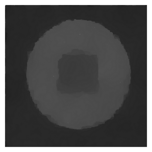
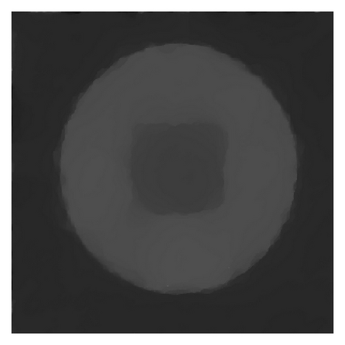
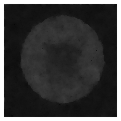
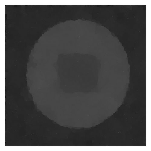
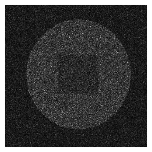
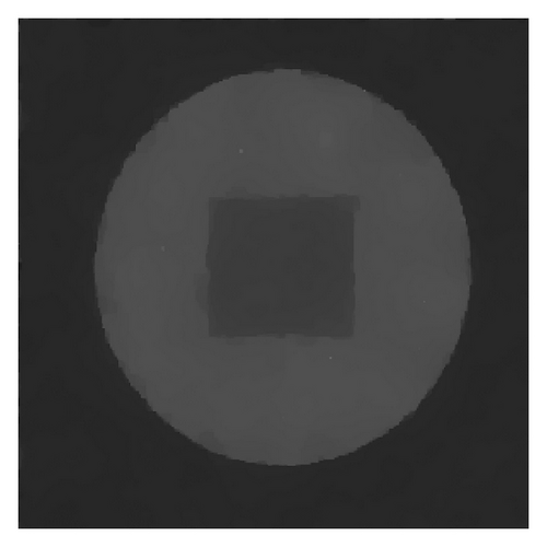
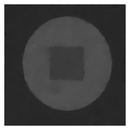
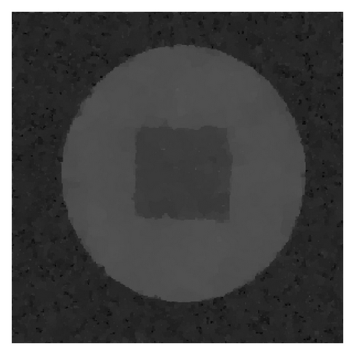
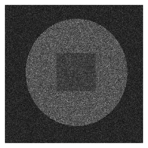
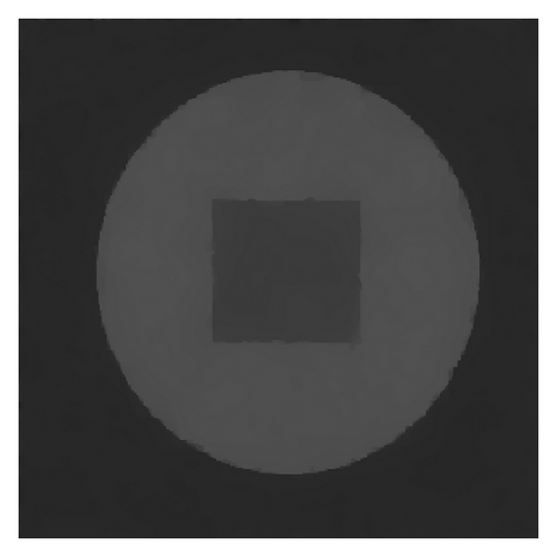
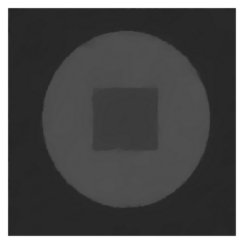
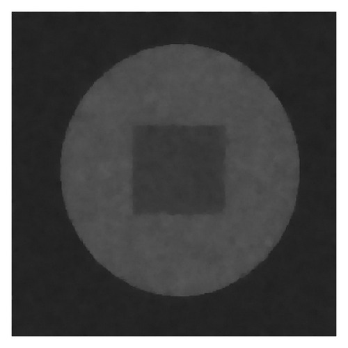
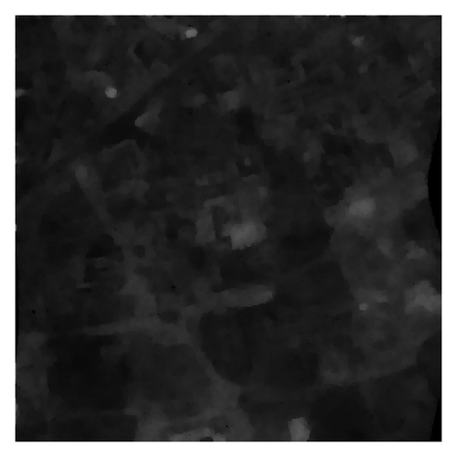
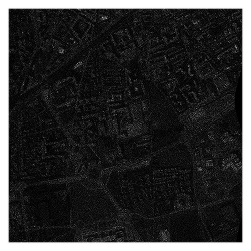
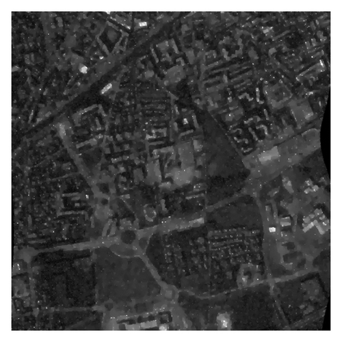
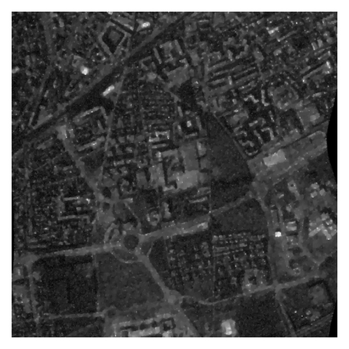
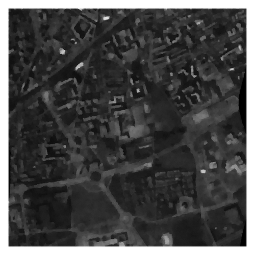
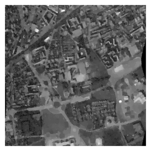
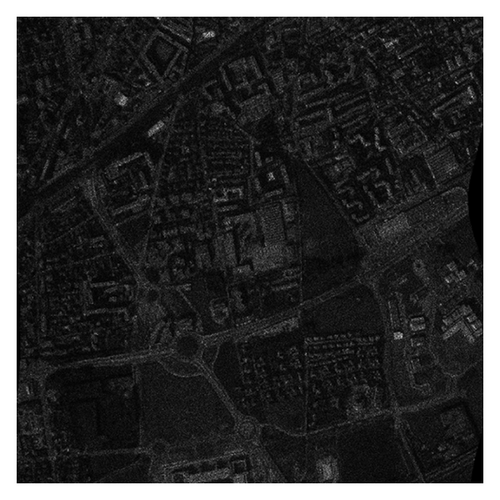
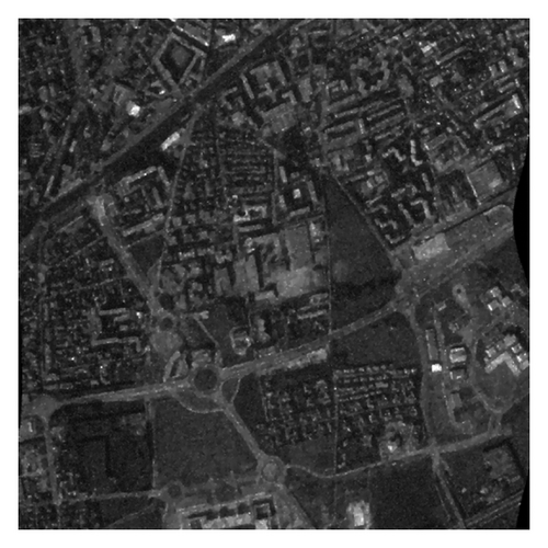
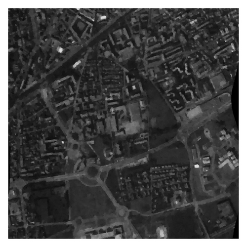
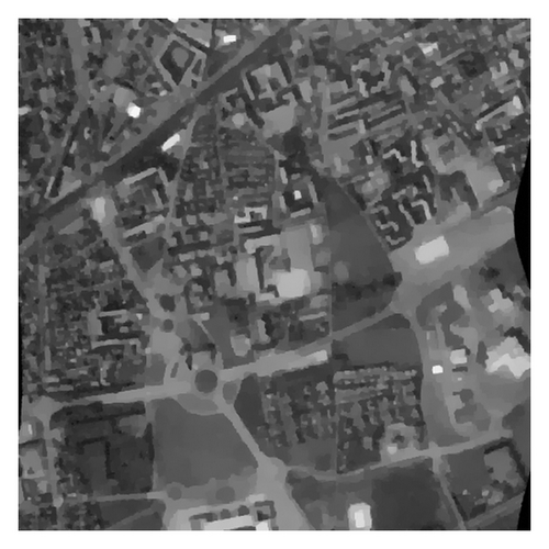
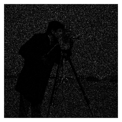
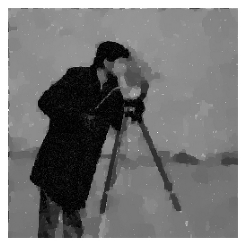
In the numerical experiments, we can see that for the nontexture image, our methods and AA method work well (see Figure 4); for the texture image, our methods and SO method work well (see Figure 7). The denoising performance results are tabulated in Table 2, where the best PSNR and MAE values are shown in boldface. The PSNR improvement brought by our approach can be quite high particularly for L = 1 (see e.g., Figures 2–4), and the visual resolution is quite respectable. This is an important achievement since in practice L has a small value, usually 1, rarely above 4. This improvement becomes less salient as L increases which is intuitively expected. But even for L = 10, the PSNR of our algorithm can be higher than AA and SO methods (see Table 2).

Table 2. PSNR and MAE.

PSNR				MAE
L	1	4	10	L	1	4	10
The synthetic image (300 × 300)

α-TV	19.67	23.86	26.37	α-TV	2.45	1.27	0.92
p-LA	19.76	23.14	25.68	p-LA	2.51	1.43	0.96
SO	4.14	15.81	21.00	SO	23.94	6.15	2.84
AA	16.33	20.14	23.94	AA	4.50	2.94	1.49

The aerial image (512 × 512)

α-TV	23.25	25.82	27.92	α-TV	12.00	8.95	7.12
p-LA	23.47	26.16	28.18	p-LA	11.64	8.81	6.98
SO	17.82	24.00	27.27	SO	25.44	11.05	7.42
AA	22.34	24.20	26.04	AA	13.35	10.30	8.13

The cameraman image (256 × 256)

α-TV	20.81	24.22	26.29	α-TV	14.65	8.88	7.14
p-LA	24.10	23.14	26.03	p-LA	13.94	9.18	7.43
SO	14.15	21.61	24.96	SO	38.92	14.64	8.36
AA	18.81	21.91	24.25	AA	22.14	14.25	9.97

Acknowledgments

The authors would like to express their sincere thanks to the referees for their valuable suggestions for the revision of the paper which contributed greatly to this work. The authors would also like to thank Jalal Fadili for providing them the MATLAB code of his algorithm. They would like to express their deep thanks to the referees for their suggestions while revising the paper, yet again. This work was partially supported by the Fundamental Research Funds for the Central Universities (Grant nos. HIT.NSRIF.2011003 and HIT.NSRIF.2012065), the National Science Foundation of China (Grant no. 11271100), the Aerospace Supported Fund, China, under Contract no. 2011-HT-HGD-06, China Postdoctoral Science Foundation funded project, Grant no. 2012M510933, and also the 985 project of Harbin Institute of Technology.

References

1 Rudin L. I., Lions P. L., and Osher S., S. Osher and N. Paragios, Multiplicative denoising and deblurring: theory and algorithms, Geometric Level Set Methods in Imaging, Vision, and Graphics, Chapter Multiplicative Denoising and De-Blurring: Theory and Algorithms, 2003, 103–120.
10.1007/0-387-21810-6_6
Google Scholar
2 Tur M., Chin C., and Goodman J. W., When is speckle noise multiplicative?, Applied Optics. (1982) 21, no. 7, 1157–1159, https://doi.org/10.1364/AO.21.001157.
10.1364/AO.21.001157
CAS PubMed Web of Science® Google Scholar
3 Goodman J. W., Statistical Properties of Laser Speckle Patterns, 1984, 11, 2nd edition, Springer, Topics in Applied Physics.
Google Scholar
4 MunsonD. C.Jr. and Visentin R. L., A signal processing view of strip-mapping synthetic aperture radar, IEEE Transactions on Accoustics, Speech, and Signal Processing. (1989) 37, no. 12, 2131–2147.
10.1109/29.45556
Web of Science® Google Scholar
5 Aubert G. and Aujol J.-F., A variational approach to removing multiplicative noise, SIAM Journal on Applied Mathematics. (2008) 68, no. 4, 925–946, https://doi.org/10.1137/060671814, MR2390974, ZBL1151.68713.
10.1137/060671814
Web of Science® Google Scholar
6 Rudin L., Osher S., and Fatemi E., Nonlinear total variation based noise removal algorithms, Physica D. (1992) 60, 259–268..
10.1016/0167-2789(92)90242-F
Web of Science® Google Scholar
7 Abramowitz M. and Stegun I. A., Handbook of Mathematical Functions, 1972, Dover, New York, NY, USA.
CAS Google Scholar
8 Shi J. and Osher S., A nonlinear inverse scale space method for a convex multiplicative noise model, SIAM Journal on Imaging Sciences. (2008) 1, no. 3, 294–321, https://doi.org/10.1137/070689954, MR2486034, ZBL1185.94018.
10.1137/070689954
Web of Science® Google Scholar
9 Darbon J., Sigelle M., and Tupin F., Contrast preservation filtering using nice-levelable functions and applications to SAR imaging, IEEE Transactions on Image Processing. (2007) .
Google Scholar
10 Rudin L. I., Lions P. L., and Osher S., S. Osher and N. Paragios, Multiplicative denoising and deblurring: theory and algorithms, Geometric Level Set Methods in Imaging, Vision, and Graphics, Chapter Multiplicative Denoising and De- Blurring: Theory and Algorithms, 2003, 103–120.
10.1007/0-387-21810-6_6
Google Scholar
11 Huang Y.-M., Ng M. K., and Wen Y.-W., A new total variation method for multiplicative noise removal, SIAM Journal on Imaging Sciences. (2009) 2, no. 1, 20–40, https://doi.org/10.1137/080712593, MR2486520.
10.1137/080712593
Web of Science® Google Scholar
12 Huang Y., Ng M. K., and Wen Y.-W., A fast total variation minimization method for image restoration, Multiscale Modeling & Simulation. (2008) 7, no. 2, 774–795, https://doi.org/10.1137/070703533, MR2443011, ZBL1172.94316.
10.1137/070703533
Web of Science® Google Scholar
13 Jin Z. and Yang X., Analysis of a new variational model for multiplicative noise removal, Journal of Mathematical Analysis and Applications. (2010) 362, no. 2, 415–426, https://doi.org/10.1016/j.jmaa.2009.08.036, MR2557697, ZBL1191.68788.
10.1016/j.jmaa.2009.08.036
Web of Science® Google Scholar
14 Strong D. M. and Chan T. F., Spatially and scale adaptive total variation based regularization and anisotropic diffusion in image processing, 1996, no. CAM96-46, Univeristy of California, Los Angeles, Calif, USA.
Google Scholar
15 Le T., Chartrand R., and Asaki T. J., A variational approach to reconstructing images corrupted by Poisson noise, Journal of Mathematical Imaging and Vision. (2007) 27, no. 3, 257–263, https://doi.org/10.1007/s10851-007-0652-y, MR2325852.
10.1007/s10851-007-0652-y
Web of Science® Google Scholar
16 Chen Y. and Rao M., Minimization problems and associated flows related to weighted p energy and total variation, SIAM Journal on Mathematical Analysis. (2003) 34, no. 5, 1084–1104, https://doi.org/10.1137/S0036141002404577, MR2001660, ZBL1038.49007.
10.1137/S0036141002404577
Web of Science® Google Scholar
17 Kornprobst P., Deriche R., and Aubert G., Image sequence analysis via partial differential equations, Journal of Mathematical Imaging and Vision. (1999) 11, no. 1, 5–26, https://doi.org/10.1023/A:1008318126505, MR1715446.
10.1023/A:1008318126505
Web of Science® Google Scholar
18 Chambolle A., An algorithm for mean curvature motion, Interfaces and Free Boundaries. (2004) 6, no. 2, 195–218, https://doi.org/10.4171/IFB/97, MR2079603, ZBL1061.35147.
10.4171/ifb/97
Web of Science® Google Scholar
19 Giusti E., Minimal Surfaces and Functions of Bounded Variation, 1994, Birkhauser.
Google Scholar
20 Chen Y., Levine S., and Rao M., Variable exponent, linear growth functionals in image restoration, SIAM Journal on Applied Mathematics. (2006) 66, no. 4, 1383–1406, https://doi.org/10.1137/050624522, MR2246061, ZBL1102.49010.
10.1137/050624522
Web of Science® Google Scholar
21 Zhou X., An evolution problem for plastic antiplanar shear, Applied Mathematics and Optimization. (1992) 25, no. 3, 263–285, https://doi.org/10.1007/BF01182324, MR1148668, ZBL0758.73014.
10.1007/BF01182324
Web of Science® Google Scholar
22 Ladyženskaja O. A., Solonnikov V. A., and Uralceva N. N., Linear and Quasilinear Equations of Parabolic Type, 1967, 23, American Mathematical Society, Providence, RI, USA, Translated from the Russian by S. Smith. Translations of Mathematical Monographs.
Google Scholar
23 Hardt R. and Zhou X., An evolution problem for linear growth functionals, Communications in Partial Differential Equations. (1994) 19, no. 11-12, 1879–1907, https://doi.org/10.1080/03605309408821076, MR1301176, ZBL0811.35061.
10.1080/03605309408821076
Web of Science® Google Scholar
24 Song B., Topics in variational PDE image segmentation, inpainting and denoising [Ph.D. thesis], 2003, University of California Los Angeles, Angeles, Calif, USA.
Google Scholar
25 Durand S., Fadili J., and Nikolova M., Multiplicative noise removal using L1 fidelity on frame coefficients, Journal of Mathematical Imaging and Vision. (2010) 36, 201–226.
10.1007/s10851-009-0180-z
Web of Science® Google Scholar

All articles

A Convex Adaptive Total Variation Model Based on the Gray Level Indicator for Multiplicative Noise Removal

Abstract

1. Introduction

1.1. Gaussian Noise

1.2. Gamma Noise

1.3. The Model Based on the Logarithm Transform

1.4. The Model Based on the Exponent Transform

2. A New Variational Model for Multiplicative Noise Removal

2.1. A Global Convex Fidelity Term

2.2. The Adaptive Total Variation Model

3. The Minimization Problem (28)

3.1. Preliminaries

3.2. Existence and Uniqueness of the Problem (28)

3.3. Comparison Principle

4. The Associated Evolution Equations (29)–(31)

4.1. Definition of a Pseudosolution to the Problems (29)–(31)

4.2. The Approximating Problem for Problems (29)–(31)

4.3. Existence and Uniqueness of the Problems (29)–(31)

4.4. Long-Time Behavior

5. Numerical Methods and Experimental Results

5.1. α-Total Variation Scheme

5.2. p-Laplace Approximate Scheme

5.3. Comparison with Other Methods

Acknowledgments

References

Figures

References

Information

About Wiley Online Library

Help & Support

Opportunities

Connect with Wiley

A Convex Adaptive Total Variation Model Based on the Gray Level Indicator for Multiplicative Noise Removal

Abstract

1. Introduction

1.1. Gaussian Noise

1.2. Gamma Noise

1.3. The Model Based on the Logarithm Transform

1.4. The Model Based on the Exponent Transform

2. A New Variational Model for Multiplicative Noise Removal

2.1. A Global Convex Fidelity Term

2.2. The Adaptive Total Variation Model

3. The Minimization Problem (28)

3.1. Preliminaries

3.2. Existence and Uniqueness of the Problem (28)

3.3. Comparison Principle

4. The Associated Evolution Equations (29)–(31)

4.1. Definition of a Pseudosolution to the Problems (29)–(31)

4.2. The Approximating Problem for Problems (29)–(31)

4.3. Existence and Uniqueness of the Problems (29)–(31)

4.4. Long-Time Behavior

5. Numerical Methods and Experimental Results

5.1. α-Total Variation Scheme

5.2. p-Laplace Approximate Scheme

5.3. Comparison with Other Methods

Acknowledgments

References

Figures

References

Related

Information