Volume 2013, Issue 1 876298

Research Article

Open Access

0-1 Test for Chaos in a Fractional Order Financial System with Investment Incentive

Corresponding Author

Baogui Xin

[email protected]

orcid.org/0000-0002-7739-4808

Nonlinear Science Center, School of Economics and Management, Shandong University of Science and Technology, Qingdao 266590, China sdust.edu.cn

Nonlinear Dynamics and Chaos Group, School of Management, Tianjin University, Tianjin 300072, China tju.edu.cn

Search for more papers by this author

Yuting Li,

Yuting Li

orcid.org/0000-0002-0951-0037

Nonlinear Science Center, School of Economics and Management, Shandong University of Science and Technology, Qingdao 266590, China sdust.edu.cn

Search for more papers by this author

Baogui Xin,

Corresponding Author

Baogui Xin

[email protected]

orcid.org/0000-0002-7739-4808

Nonlinear Science Center, School of Economics and Management, Shandong University of Science and Technology, Qingdao 266590, China sdust.edu.cn

Nonlinear Dynamics and Chaos Group, School of Management, Tianjin University, Tianjin 300072, China tju.edu.cn

Search for more papers by this author

Yuting Li,

Yuting Li

orcid.org/0000-0002-0951-0037

Nonlinear Science Center, School of Economics and Management, Shandong University of Science and Technology, Qingdao 266590, China sdust.edu.cn

Search for more papers by this author

First published: 11 November 2013

https://doi.org/10.1155/2013/876298

Citations: 30

Academic Editor: Luca Guerrini

Share a link

Email
Wechat
Bluesky

Abstract

A new integer-order chaotic financial system is extended by introducing a simple investment incentive into a three-dimensional chaotic financial system. A four-dimensional fractional-order chaotic financial system is presented by bringing fractional calculus into the new integer-order financial system. By using weighted integral thought, the fractional order derivative′s economics meaning is given. The 0-1 test algorithm and the improved Adams-Bashforth-Moulton predictor-corrector scheme are employed to detect numerically the chaos in the proposed fractional order financial system.

1. Introduction

In recent years there has been a high level of interest in the study of chaotic economic systems [1, 2]. Chaotic systems refer to nonlinear dynamical systems which are very sensitive to initial conditions, in a such way that a small perturbation of these could have unpredictable consequences on the evolution equations. As a complex system, the financial system shows a lot of nonlinear dynamical phenomena, such as chaos, fractals, and bifurcation. Reference [3] firstly presented a nonlinear financial model as follows:

()

where x denotes the interest rate, y denotes the investment demand, z denotes the price index, a is the saving amount, b is the cost per investment, c is the demand elasticity of commercial markets, and all three constants a, b, c ≥ 0.

References [4–7] analyzed some complex behavior of system (1), such as bifurcation and chaos. Reference [8] introduced fractional calculus into system (1) and studied its complex dynamics [9]. References [10, 11] studied chaos control of the fractional-order form of system (1). Reference [12] proposed an uncertain fractal-order form of system (1) and studied its chaos control via adaptive sliding mode. Reference [13] proposed an uncertain and stochastic form of system (1) with multiple delays. Reference [14] proposed a discrete form of system (1) and studied its Neimark-Sacker bifurcation. References [15, 16] presented a form of system (1) with time-delayed feedback and studied its dynamics and control. Reference [17] studied Hopf-pitchfork bifurcation and periodic phenomena in the system (1) with time delays. Reference [18] extended system (1) with the average profit margin.

Investment is an important economic activity [19]. In order to cope with high unemployment or backwardness, in many cases a government would use their policies to stimulate investment which will raise employment, exports, tax revenue, and so on. These incentives may take the form of investment grants or investment credit that reduces capital costs for investors. But these various forms of investment incentives also will arouse the investment demand of the financial system (1). In other words, there may be a positive feedback mechanism between investment command and investment incentive. Thus we can describe the above mechanism by using the following four-dimensional financial system with a simple investment incentive:

()

where x, y, z, a, b, and c have the same meanings as those defined in the system (1), u denotes the investment incentive, and d ≥ 0 is the coefficient of investment incentive intensity.

Researchers’ ever-growing interests in fractional calculus have led the ever-broadening applications in a lot of fields [20–25]. When fractional calculus is introduced into the system (2), its fractional-order form can be described with fractional derivative as follows:

()

in which q = (q₁, q₂, q₃, q₄) is subject to 0 < q₁, q₂, q₃, q₄ < 1.

Remark 1. When q = (1,1, 1,1), the system (3) degenerates into the system (2).

The remainder of this paper is organized as follows. In Section 2, we give some preliminaries, such as Caputo fractional derivative’s economics meaning, numerical solutions of the system (3), and the 0-1 test algorithm. In Section 3, we numerically illustrate the chaos existence of the proposed financial system by using the improved Adams-Bashforth-Moulton predictor-corrector scheme and 0-1 test algorithm. Finally conclusions in Section 4 close the paper.

2. Preliminaries

2.1. Caputo Fractional Derivative and Its Economics Meaning

2.1.1. Weighted Integral

The integer integral and derivative are very helpful to understand fractional integral and derivative. An integral can be thought of as an area or a generalization of area.

Definition 2. Given a weighted factor f(x) and a function g(x) for a ≤ x ≤ b, the definite weighted integral is a real number whose geometrical interpretation is the signed area under the graph of weighted function y = f(x)g(x) for a ≤ x ≤ b.

The Riemann integral is a simple and well-understood integral definition. If the continuous function g(x) is defined on interval [a, b] and a partition P of [a, b] can be divided into a collection of subintervals [x₀, x₁], [x₁, x₂], …, [x_n−1, x_n], for each i = 1,2, …, n, a point

in [x_n−1, x_n], and its weighted factor

, weighted Riemann integral

can be rewritten as

()

for any choice of the

in [x_n−1, x_n] with Δx = (b − a)/n and x_i = a + iΔx.

When f(x) = 1, the weighted integral completely degenerates into a common integral.

2.1.2. Caputo Fractional Derivative

Loosely speaking, a derivative can be interpreted as a kind of change ratio. More specifically it is the measure of infinitesimal change ratio of the output over the infinitesimal change of the input. For example, consider the following.

Definition 3. The first order derivative of function f(t) with respect to t is given by

()

Definition 4. The 2nd order derivative of function f(t) with respect to t is given by

()

Definition 5. The mth order derivative of function f(t) with respect to t is given by

()

And there are several definitions of fractional derivatives, roughly speaking, which can be thought of as generalized above derivatives. The Caputo definition is a common notation of fractional derivative. Briefly the Caputo fractional derivative is a kind of weighted change ratio in a time interval. More specifically, the Caputo fractional derivative can be considered as a kind of weighted integral of the integer order derivative of a function on an interval. In this paper, we will adopt the following Caputo definition.

Definition 6. The qth order fractional derivative of function f(t) with respect to t is given by

()

where K_q(t − τ) = (t − τ) ^m−q−1/Γ(m − q),

, t ∈ [a, b], m is an integer and m − 1 < q ≤ m.

The functions f^(m)(t) in Definitions 5 and 6 are the same. When K_q(t − τ) is regarded as a kind of weight, then can be regarded as a kind of weighted integral with respect to f^(m)(t). What is more, f^(m)(t) can be regarded as mth order change ratio of the function f(t) at t; that is, there is no memory effect in f^(m)(t). However, can be regarded as a weighted integral of the mth order derivative of the function f(t) on the whole interval [a, b], and the weight K_q(t − τ) depends on the specific time; that is, there are memory effects in .

2.1.3. Caputo Fractional Derivative’s Economics Meaning

In economics, let me illustrate a concrete example like the system (3), for the investment demand function y(t), its integer order derivative y^(m)(t), and its fractional order derivative , y^(m)(t) can be regarded as mth order change ratio of the investment demand y(t) at the time t; that is, it is unrelated to any time before the time t; that is, there is no memory effect in y^(m)(t). However, can be regarded as a weighted integral of all mth order derivative of the investment demand y(t) on the whole time interval [0, t]; that is, does not only depend on the time t, but also depends on any time before the time t; that is, there are memory effects in . In the system (3), m = 1 and its memory effects are easier to be understood, so we will not repeat them here. In fact, a lot of economics variables have memory effects; for example, our past economic behavior may affect our present and future ones. In other research fields, there are also a lot of memory effects, such as psychological shadow, escalation of commitment, sunk cost effect, lazy battery effect, and shape memory effect. As mentioned above, there are some memory effects in financial systems, so the fractional derivative may be more suitable to study them.

2.2. Numerical Solutions of Fractional Order System

Based on the improved Adams-Bashforth-Moulton predictor-corrector scheme [26–29], one can solve fractional-order ordinary differential equations. The numerical calculation formula of fractional-order system (3) can be described as follows.

With the initial value

, k = 0,1, …, [m] − 1, and the fractional-order system (3) is equivalent to the Volterra integral equations as follows:

()

Let h = T/N, t_n = nh, n = 0,1, …, N ∈ Z⁺, and the fractional-order system (3) can be approximated to the following difference equations:

()

where

()

Errors of the above method are

()

where p_i = min (2,1 + q_i).

2.3. The 0-1 Test Algorithm

There are many approaches to detect chaos, but 0-1 test is one of the simplest and most effective ones, which was proposed by Gottwald and Melbourne [30] and also has already been successfully tested for various discrete or continuous systems, such as [31–45].

In this section, we introduce the detailed steps of the 0-1 test algorithm to robustly distinguish regular from chaotic dynamics in deterministic continuous dynamical systems. In fact, one can directly implement the 0-1 test algorithm if the given time series is generated from a discrete time system. But if the given time series is generated from a continuous time system, there may be a well-known oversampling issue that must overcome it. So the oversampling issue should be considered when we distinguish regular from chaotic dynamic system (3).

Consider a set of measurement data ϕ₀(i) obtained from a continuous time system, where i = 1,2, …,T, and T is the amount of the data, the 0-1 test algorithm can be described as follows.

Step 1. Rearrange the initial measurement data with an optimal sampling time.

The average mutual information [46] between ϕ₀(i) and ϕ₀(i + τ) is defined as

()

where τ is the time delay, that is, sampling time.

The value τ corresponding to the first local minimum of the mutual information I(τ) is the optimal sampling time. Thus we can rearrange the initial measurement data ϕ₀(i) into the finely sampled measurement data ϕ(j) in the following way:

()

where i = 1,2, …, T, and j = 1,2, 3, …, N.

Step 2. Choose a random number c ∈ (π/5, 4π/5) and define the following new coordinates (p_c(n), s_c(n)):

()

where

()

Step 3. Define the mean square displacement M_c(n) as follows:

()

Step 4. Define the modified mean square displacement D_c(n) as follows:

()

Step 5. Define the median value of correlation coefficient K as follows:

()

where

()

in which ξ = (1,2, 3, …, n_cut), Δ = (D_c(1), D_c(2), …, D_c(n_cut)), n_cut = round(N/10), and the covariance and variance are defined with vectors x, y of length q as follows:

()

Step 6. Interpret outputs as follows.

(1)
K ≈ 0 indicates the underlying dynamics is regular (i.e., periodic or quasiperiodic), whereas K ≈ 1 indicates the underlying dynamics is chaotic.
(2)
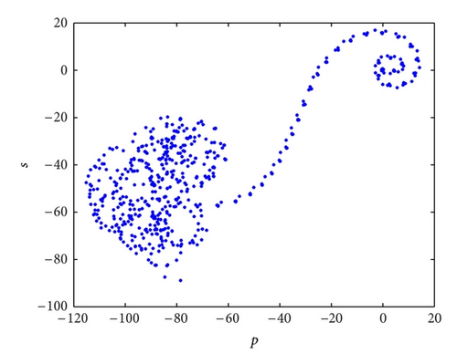
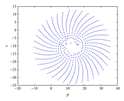
Bounded trajectories in the (p, s) plane imply the underlying dynamics is regular (i.e., periodic or quasiperiodic), whereas Brownian-like (unbounded) trajectories imply the underlying dynamics is chaotic.

3. Some Basic Properties of the System (3)

3.1. Symmetry and Invariance

Obviously, the four-dimensional system (3) has a natural symmetry about the coordinate plane y-u since the coordinate transformation (x, y, z, u)→(−x, y, −z, u) satisfies the system is invariant for all values of the system parameters.

3.2. Dissipativity and the Existence of Attractor

From system (3), we obtain

()

that is, the system (3) is dissipative with an exponential contraction rate dV/dt = e^−(a+b+c) when a + b + c > 0. In other words, the volume element V(t) = V₀e^−(a+b+c)t for the initial volume V₀ means the trajectories of chaotic system (3) would converge ultimately onto an attractor as t → ∞ with an exponential rate (a + b + c).

3.3. Equilibrium and Stability

Theorem 7 (see [47].)Consider a nonlinear autonomous fractional order system as follows:

()

where

, and 0 < q_i < 1 (i = 1,2, …, n). If

is the jacobian matrix at its equilibrium

, then the point

is asymptotically stable when |arg( eig (A))| > q_mπ/2, where q_m = max _1≤i≤n{q_i}.

The equilibrium of the system (3) satisfies the following equations:

()

By simple computation, one can obtain that system (3) has only one equilibrium point E₀(0,0, 0, −1).

Proposition 8. The equilibrium point E₀ is unstable.

Proof. For the equilibrium point E₀, the Jacobian matrix is

()

It is easy to get its eigenvalues corresponding to the equilibrium J(E₀) as follows: , , , and .

Obviously λ₁ > 0, that is, |arg(λ₁)| = 0, thus the equilibrium point E₀ is unstable based on Theorem 7.

This proposition is proved.

4. 0-1 Test for Chaos in the System (3)

In the next two subsections, some properties of the system (3) will be, respectively, discussed by varying investment incentive intensity d and investment demand derivative q₂. The abovementioned Adams-Bashforth-Moulton predictor-corrector scheme and 0-1 test algorithm can be employed to get the desired numerical solutions of system (3).

4.1. Varying d and Fixing q₁ = 0.96, q₂ = 0.94, q₃ = 0.92, q₄ = 0.78, a = 3, b = 0.4, and c = 0.4

To simplify representation, one can fix q₁ = 0.96, q₂ = 0.94, q₃ = 0.92, q₄ = 0.78, a = 3, b = 0.4, and c = 0.4 in this subsection. When the investment incentive intensity d varies, the corresponding K values are shown in Figure 1(a). The bifurcation diagram of interest rate x with increasing the investment incentive intensity d is presented in Figure 1(b). Obviously the bifurcation diagram well coincides with the K diagram. The two abovementioned figures both show that system (3) changes gradually from chaos to stability as the investment incentive intensity d grows larger.

Details are in the caption following the image — **Figure 1 (a) 0-1 test with K versus d**
Open in figure viewer PowerPoint

The evolvement of K and x versus d with q₁ = 0.96, q₂ = 0.94, q₃ = 0.92, q₄ = 0.78, a = 3, b = 0.4, and c = 0.4.

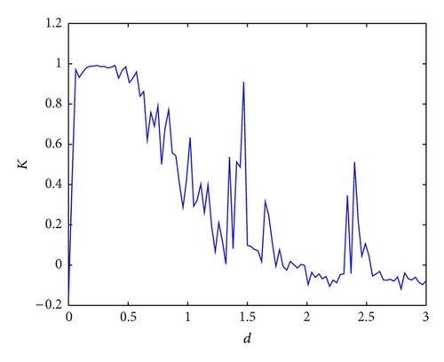
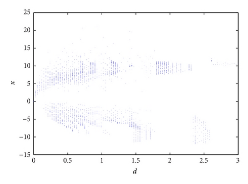
From Figure 1, the complex dynamical behavior of the system (3) can be clearly understood. When the investment incentive intensity d is determined by its corresponding K ≈ 1, the system (3) is chaotic. Whereas the investment incentive intensity d is determined by its corresponding K ≈ 0, the system (3) is regular.

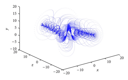
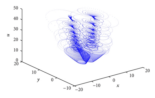
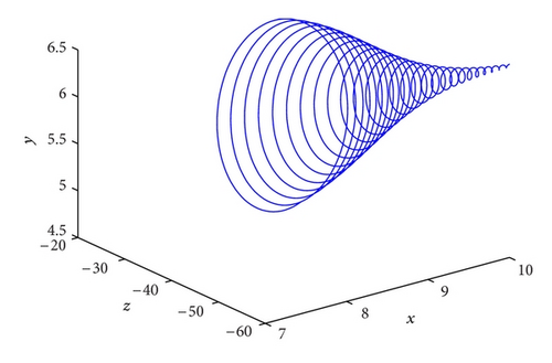
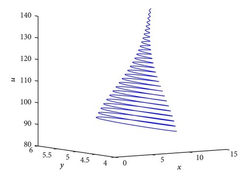
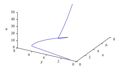
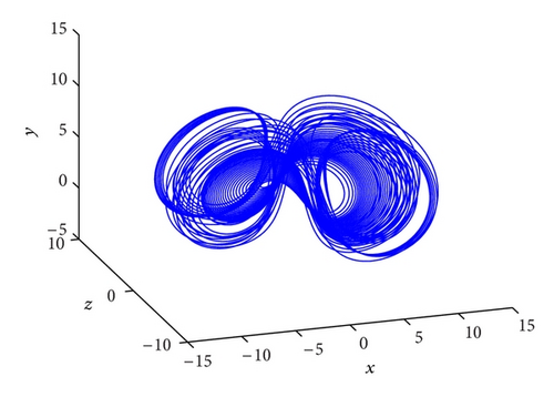
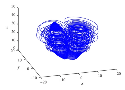
Let me take two specific examples as illustrations in the system (3). When the investment incentive intensity d = 0.1, its corresponding phase portraits are strange attractors as shown in Figure 2 and its trajectories in the new (p, s)-plane are Brownian-like as shown in Figure 3(a); that is, the system (3) is chaotic. Whereas the investment incentive intensity d = 2.8, its corresponding phase portraits are quasiperiodic as shown in Figure 4 and its trajectories in the new (p, s) plane are bounded as shown in Figure 3(b); that is, the system (3) is regular (quasiperiodic).

4.2. Varying q₂ and Fixing q₁ = 0.98, q₃ = 0.97, q₄ = 0.78, a = 3, b = 0.4, c = 0.4, d = 0.1

In the following subsection, q₁ = 0.98, q₃ = 0.97, q₄ = 0.78, a = 3, b = 0.4, c = 0.4, d = 0.1 are fixed. When d varies, the corresponding K values are shown in Figure 5(a). The bifurcation diagram of interest rate x with increasing the investment demand derivative q₂ is given in Figure 5(b). Obviously the bifurcation diagram well coincides with the K diagram, too. Figure 5 shows that the system (3) changes gradually from stability to chaos as the investment demand derivative q₂ grows larger.

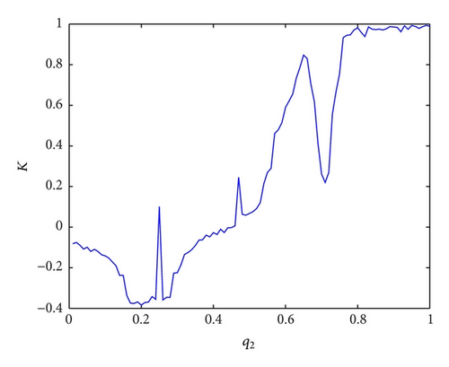
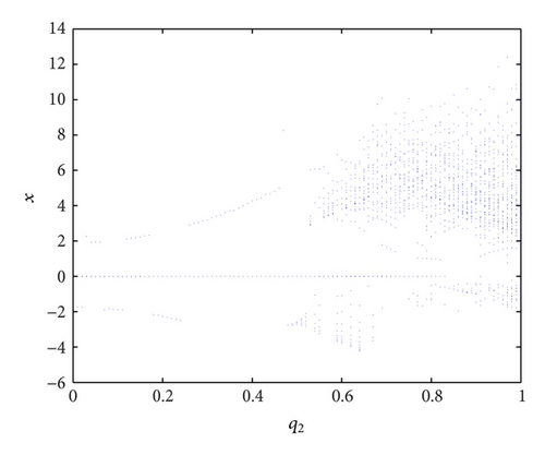
From Figure 5 of the system (3), when the investment demand derivative q₂ is determined by its corresponding K ≈ 1, the system (3) is chaotic. Whereas the investment demand derivative q₂ is determined by its corresponding K ≈ 0, the system (3) is regular.

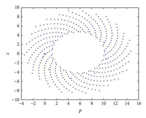
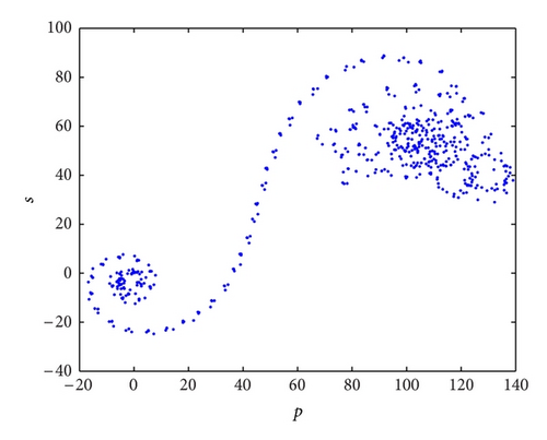
For example, in the system (3), when the investment demand derivative q₂ = 0.4, its corresponding phase portraits are quasiperiodic as shown in Figure 7 and its trajectories in the (p, s) plane are bounded as shown in Figure 6(a); that is, the system (3) is regular (quasiperiodic). Whereas the investment demand derivative q₂ = 0.89, its corresponding phase portraits are strange attractors as shown in Figure 8 and its trajectories in the (p, s) plane are Brownian-like as shown in Figure 6(b); that is, the system (3) is chaotic.

5. Conclusion

A government is used to employing investment incentive to regulate financial systems. In this paper, a simple investment incentive is introduced into the classical chaotic financial system, and a 4-D chaotic financial system is obtained. What is more, there are some memory effects in the financial systems, so the 4-D fractional-order chaotic financial system is proposed by introducing the fractional calculus into the mentioned 4-D integer-order financial system. With the improved Adams-Bashforth-Moulton predictor-corrector scheme, phase portraits and bifurcation diagrams are illustrated, and then K value diagram and Plots in new coordinates (p, s) space are given by using the 0-1 test algorithm. Thus chaotic dynamics is distinguished from regular dynamics in the 4-D fractional-order chaotic financial system by the abovementioned methods.

Conflict of Interests

The authors declare that there is no conflict of interests regarding the publication of this paper.

Acknowledgments

This work is supported partly by Excellent Young Scientist Foundation of Shandong Province (Grant no. BS2011SF018), National Social Science Foundation of China (Grant no. 12BJY103), Humanities and Social Sciences Foundation of the Ministry of Education of China (Grant no. 11YJCZH200), and National Natural Science Foundation of China (Grant no. 71272148).

References

1 Chian A. C.-L., Rempel E. L., and Rogers C., Complex economic dynamics: chaotic saddle, crisis and intermittency, Chaos, Solitons and Fractals. (2006) 29, no. 5, 1194–1218, 2-s2.0-33646530978, https://doi.org/10.1016/j.chaos.2005.08.218.
10.1016/j.chaos.2005.08.218
Web of Science® Google Scholar
2 Xin B., Ma J., and Gao Q., The complexity of an investment competition dynamical model with imperfect information in a security market, Chaos, Solitons and Fractals. (2009) 42, no. 4, 2425–2438, 2-s2.0-67650844274, https://doi.org/10.1016/j.chaos.2009.03.110.
10.1016/j.chaos.2009.03.110
Web of Science® Google Scholar
3 Huang D. and Li H., Theory and Method of the Nonlinear Economics, 1993, Sichuan University, Chengdu, China, (Chinese).
Google Scholar
4 Ma J.-H. and Chen Y.-S., Study for the bifurcation topological structure and the global complicated character of a kind of nonlinear finance system (I), Applied Mathematics and Mechanics. (2001) 22, no. 11, 1240–1251, 2-s2.0-0035502834, https://doi.org/10.1023/A:1016313804297.
10.1023/A:1016313804297
Web of Science® Google Scholar
5 Ma J.-H. and Chen Y.-S., Study for the bifurcation topological structure and the global complicated character of a kind of nonlinear finance system (II), Applied Mathematics and Mechanics. (2001) 22, no. 12, 1375–1382, 2-s2.0-0035741173, https://doi.org/10.1023/A:1022806003937.
10.1023/A:1022806003937
Web of Science® Google Scholar
6 Ma J. and Bangura T., Complexity analysis research of financial and economic system under the condition of three parameters change circumstances, Nonlinear Dynamics. (2012) 70, 2313–2326.
10.1007/s11071-012-0336-z
Web of Science® Google Scholar
7 Gao Q. and Ma J., Chaos and Hopf bifurcation of a finance system, Nonlinear Dynamics. (2009) 58, no. 1-2, 209–216, 2-s2.0-70349215638, https://doi.org/10.1007/s11071-009-9472-5.
10.1007/s11071-009-9472-5
Web of Science® Google Scholar
8 Chen W.-C., Nonlinear dynamics and chaos in a fractional-order financial system, Chaos, Solitons and Fractals. (2008) 36, no. 5, 1305–1314, 2-s2.0-38649117916, https://doi.org/10.1016/j.chaos.2006.07.051.
10.1016/j.chaos.2006.07.051
Web of Science® Google Scholar
9 Xin B.-G., Chen T., and Liu Y.-Q., Complexity evolvement of a chaotic fractional-order financial system, Acta Physica Sinica. (2011) 60, no. 4, 2-s2.0-79955508569, 048901.
10.7498/aps.60.048901
Web of Science® Google Scholar
10 Abd-Elouahab M. S., Hamri N.-E., and Wang J., Chaos control of a fractional-order financial system, Mathematical Problems in Engineering. (2010) 2010, 18, 2-s2.0-77955296664, https://doi.org/10.1155/2010/270646, 270646.
10.1155/2010/270646
Web of Science® Google Scholar
11 Pan I., Korre A., Das S., and Durucan S., Chaos suppression in a fractional order financial system using intelligent regrouping PSO based fractional fuzzy control policy in the presence of fractional Gaussian noise, Nonlinear Dynamics. (2012) 70, 2445–2461.
10.1007/s11071-012-0632-7
Web of Science® Google Scholar
12 Wang Z., Huang X., and Shen H., Control of an uncertain fractional order economic system via adaptive sliding mode, Neurocomputing. (2012) 83, 83–88, 2-s2.0-84856604260, https://doi.org/10.1016/j.neucom.2011.11.018.
10.1016/j.neucom.2011.11.018
Web of Science® Google Scholar
13 Mircea G., Neamtu M., Bundau O., and Opris D., Uncertain and stochastic financial models with multiple delays, International Journal of Bifurcation and Chaos. (2012) 22, no. 6, 19, 1250131, https://doi.org/10.1142/S0218127412501313.
10.1142/S0218127412501313
Web of Science® Google Scholar
14 Xin B., Chen T., and Ma J., Neimark-sacker bifurcation in a discrete-time financial system, Discrete Dynamics in Nature and Society. (2010) 2010, 12, 2-s2.0-77957856904, https://doi.org/10.1155/2010/405639, 405639.
10.1155/2010/405639
Web of Science® Google Scholar
15 Chen W.-C., Dynamics and control of a financial system with time-delayed feedbacks, Chaos, Solitons and Fractals. (2008) 37, no. 4, 1198–1207, 2-s2.0-40749160977, https://doi.org/10.1016/j.chaos.2006.10.016.
10.1016/j.chaos.2006.10.016
Web of Science® Google Scholar
16 Son W.-S. and Park Y.-J., Delayed feedback on the dynamical model of a financial system, Chaos, Solitons and Fractals. (2011) 44, no. 4-5, 208–217, 2-s2.0-79955019125, https://doi.org/10.1016/j.chaos.2011.01.010.
10.1016/j.chaos.2011.01.010
Web of Science® Google Scholar
17 Ding Y., Jiang W., and Wang H., Hopf-pitchfork bifurcation and periodic phenomena in nonlinear financial system with delay, Chaos, Solitons & Fractals. (2012) 45, 1048–1057.
10.1016/j.chaos.2012.05.006
Web of Science® Google Scholar
18 Yu H., Cai G., and Li Y., Dynamic analysis and control of a new hyperchaotic finance system, Chaos, Solitons & Fractals. (2012) 45, 1048–1057.
Google Scholar
19 Dinica M., The real options attached to an investment project, Economia, Seria Management. (2011) 14, 511–518.
Google Scholar
20 Xin B., Chen T., and Liu Y., Synchronization of chaotic fractional-order WINDMI systems via linear state error feedback control, Mathematical Problems in Engineering. (2010) 2010, 10, 2-s2.0-77957833830, https://doi.org/10.1155/2010/859685, 859685.
10.1155/2010/859685
Web of Science® Google Scholar
21 Xin B., Chen T., and Liu Y., Projective synchronization of chaotic fractional-order energy resources demand-supply systems via linear control, Communications in Nonlinear Science and Numerical Simulation. (2011) 16, no. 11, 4479–4486, 2-s2.0-79957881732, https://doi.org/10.1016/j.cnsns.2011.01.021.
10.1016/j.cnsns.2011.01.021
Web of Science® Google Scholar
22 Li X. C. and Chen W., Nested meshes for numerical approximation of space fractional differential equations, The European Physical Journal. (2011) 193, no. 1, 221–228, 2-s2.0-79953710862, https://doi.org/10.1140/epjst/e2011-01393-3.
10.1140/epjst/e2011-01393-3
Web of Science® Google Scholar
23 Li X. and Chen W., Analytical study on the fractional anomalous diffusion in a half-plane, Journal of Physics A. (2010) 43, no. 49, 2-s2.0-78649692474, https://doi.org/10.1088/1751-8113/43/49/495206, 495206.
10.1088/1751-8113/43/49/495206
Google Scholar
24 Chen S. and Jiang X., Analytical solutions to time-fractional partial differential equations in a two-dimensional multilayer annulus, Physica A. (2012) 391, no. 15, 3865–3874, 2-s2.0-84860531430, https://doi.org/10.1016/j.physa.2012.03.014.
10.1016/j.physa.2012.03.014
Web of Science® Google Scholar
25 Jiang X. and Qi H., Thermal wave model of bioheat transfer with modified Riemann-Liouville fractional derivative, Journal of Physics A. (2012) 45, 485101.
10.1088/1751-8113/45/48/485101
Google Scholar
26 Deng W., Numerical algorithm for the time fractional Fokker-Planck equation, Journal of Computational Physics. (2007) 227, no. 2, 1510–1522, 2-s2.0-36149001762, https://doi.org/10.1016/j.jcp.2007.09.015.
10.1016/j.jcp.2007.09.015
Web of Science® Google Scholar
27 Deng W., Smoothness and stability of the solutions for nonlinear fractional differential equations, Nonlinear Analysis: Theory, Methods and Applications. (2010) 72, no. 3-4, 1768–1777, 2-s2.0-71549156256, https://doi.org/10.1016/j.na.2009.09.018.
10.1016/j.na.2009.09.018
Web of Science® Google Scholar
28 Diethelm K., Ford N. J., and Freed A. D., Detailed error analysis for a fractional Adams method, Numerical Algorithms. (2004) 36, no. 1, 31–52, 2-s2.0-4043121080, https://doi.org/10.1023/B:NUMA.0000027736.85078.be.
10.1023/B:NUMA.0000027736.85078.be
Web of Science® Google Scholar
29 Diethelm K., Ford N. J., and Freed A. D., A predictor-corrector approach for the numerical solution of fractional differential equations, Nonlinear Dynamics. (2002) 29, no. 1–4, 3–22, 2-s2.0-0036650479, https://doi.org/10.1023/A:1016592219341.
10.1023/A:1016592219341
Web of Science® Google Scholar
30 Gottwald G. A. and Melbourne I., A new test for chaos in deterministic systems, Proceedings of the Royal Society A. (2004) 460, no. 2042, 603–611, 2-s2.0-1542512469, https://doi.org/10.1098/rspa.2003.1183.
10.1098/rspa.2003.1183
Google Scholar
31 Gottwald G. A. and Melbourne I., On the implementation of the 0-1 test for chaos, SIAM Journal on Applied Dynamical Systems. (2009) 8, no. 1, 129–145, 2-s2.0-63049133335, https://doi.org/10.1137/080718851.
10.1137/080718851
Web of Science® Google Scholar
32 Gottwald G. A. and Melbourne I., On the validity of the 0-1 test for chaos, Nonlinearity. (2009) 22, no. 6, 1367–1382, 2-s2.0-67650723434, https://doi.org/10.1088/0951-7715/22/6/006.
10.1088/0951-7715/22/6/006
Web of Science® Google Scholar
33 Falconer I., Gottwald G. A., Melbourne I., and Wormnes K., Application of the 0-1 test for chaos to experimental data, SIAM Journal on Applied Dynamical Systems. (2007) 6, no. 2, 395–402, 2-s2.0-57249111948, https://doi.org/10.1137/060672571.
10.1137/060672571
Web of Science® Google Scholar
34 Devi S., Singh S., and Sharma A., Deterministic dynamics of the magnetosphere: results of the 0-1 test, Nonlinear Processes in Geophysics. (2013) 20, 11–18.
10.5194/npg-20-11-2013
Web of Science® Google Scholar
35 Litak G., Syta A., and Wiercigroch M., Identification of chaos in a cutting process by the 0-1 test, Chaos, Solitons and Fractals. (2009) 40, no. 5, 2095–2101, 2-s2.0-65549143858, https://doi.org/10.1016/j.chaos.2007.09.093.
10.1016/j.chaos.2007.09.093
Web of Science® Google Scholar
36 Litak G., Syta A., Budhraja M., and Saha L. M., Detection of the chaotic behaviour of a bouncing ball by the 0-1 test, Chaos, Solitons and Fractals. (2009) 42, no. 3, 1511–1517, 2-s2.0-67650642312, https://doi.org/10.1016/j.chaos.2009.03.048.
10.1016/j.chaos.2009.03.048
Web of Science® Google Scholar
37 Bernardini D., Rega G., Litak G., and Syta A., Identification of regular and chaotic isothermal trajectories of a shape memory oscillator using the 0-1 test, Journal of Multi-Body Dynamics K. (2013) 227, no. 1, 17–22, https://doi.org/10.1177/1464419312447498.
10.1177/1464419312447498
Google Scholar
38 Sun K., Liu X., and Zhu C., The 0-1 test algorithm for chaos and its applications, Chinese Physics B. (2010) 11, 110510.
10.1088/1674-1056/19/11/110510
Google Scholar
39 Yuan L.-G. and Yang Q.-G., A proof for the existence of chaos in diffusively coupled map lattices with open boundary conditions, Discrete Dynamics in Nature and Society. (2011) 2011, 16, 2-s2.0-84855523348, https://doi.org/10.1155/2011/174376, 174376.
10.1155/2011/174376
Web of Science® Google Scholar
40 Webel K., Chaos in German stock returns—new evidence from the 0-1 test, Economics Letters. (2012) 115, no. 3, 487–489, 2-s2.0-84856077784, https://doi.org/10.1016/j.econlet.2011.12.110.
10.1016/j.econlet.2011.12.110
Web of Science® Google Scholar
41 Zachilas L. and Psarianos I. N., Examining the chaotic behavior in dynamical systems by means of the 0-1 test, Journal of Applied Mathematics. (2012) 2012, 14, 681296, https://doi.org/10.1155/2012/681296.
10.1155/2012/681296
Google Scholar
42 Xin B. and Li Y., Bifurcation and chaos in a price game of irrigation water in a coastal irrigation district, Discrete Dynamics in Nature and Society. (2013) 2013, 10, 408904, https://doi.org/10.1155/2013/408904.
10.1155/2013/408904
Web of Science® Google Scholar
43 Vahedi S. and Noorani M. S. M., Analysis of a new quadratic 3D chaotic attractor, Abstract and Applied Analysis. (2013) 2013, 7, 540769, https://doi.org/10.1155/2013/540769.
10.1155/2013/540769
Google Scholar
44 Krese B. and Govekar E., Nonlinear analysis of laser droplet generation by means of 0-1 test for chaos, Nonlinear Dynamics. (2012) 67, no. 3, 2101–2109, 2-s2.0-84855782868, https://doi.org/10.1007/s11071-011-0132-1.
10.1007/s11071-011-0132-1
Web of Science® Google Scholar
45 Kim Y., Identification of dynamical states in stimulated Izhikevich neuron models by using a 0-1 test, Journal of the Korean Physical Society. (2010) 57, no. 6, 1363–1368, 2-s2.0-78650385249, https://doi.org/10.3938/jkps.57.1363.
10.3938/jkps.57.1363
Web of Science® Google Scholar
46 Fraser A. M. and Swinney H. L., Independent coordinates for strange attractors from mutual information, Physical Review A. (1986) 33, no. 2, 1134–1140, 2-s2.0-34548696055, https://doi.org/10.1103/PhysRevA.33.1134.
10.1103/PhysRevA.33.1134
CAS PubMed Web of Science® Google Scholar
47 Yu Y., Li H.-X., Wang S., and Yu J., Dynamic analysis of a fractional-order Lorenz chaotic system, Chaos, Solitons and Fractals. (2009) 42, no. 2, 1181–1189, 2-s2.0-67649861441, https://doi.org/10.1016/j.chaos.2009.03.016.
10.1016/j.chaos.2009.03.016
Web of Science® Google Scholar

Citing Literature

All articles

0-1 Test for Chaos in a Fractional Order Financial System with Investment Incentive

Abstract

1. Introduction

2. Preliminaries