We examine possible approximate solutions of both integer and noninteger systems of nonlinear differential equations describing tuberculosis disease population dynamics. The approximate solutions are obtained via the relatively new analytical technique, the homotopy decomposition method (HDM). The technique is described and illustrated with numerical example. The numerical simulations show that the approximate solutions are continuous functions of the noninteger-order derivative. The technique used for solving these problems is friendly, very easy, and less time consuming.

1. Introduction

Tuberculosis, MTB, or TB (short for tubercle bacillus) is a common and in many cases lethal, infectious disease caused by various strains of Mycobacterium, usually Mycobacterium Tuberculosis [1]. Tuberculosis typically attacks the lungs, but can also affect other parts of the body. It is spread through the air when people who have an active TB infection cough, sneeze, or otherwise transmit their saliva through the air [2]. Most infections are asymptomatic and latent, but about one in ten latent infections eventually progresses to active disease which, if left untreated, kills more than 50% of those so infected. Interested reader can find more about this model in [3–7].

Based on the standard SIRS model, the model population was compartmentalised into the susceptible (S) and the infected (I) which is further broken down into latently infected (I_L) and actively infected (I_A) while the recovered subpopulation is ploughed back into the susceptible group due to the possibility of reinfection after successful treatment of the earlier infection. The model monitors the temporary dynamics in the population of susceptible people (t), TB latently infected people I_L(t), and TB actively infected people I_A(t) as captured in the model system of ordinary differential equations that follows.

()

subject to the initial conditions

()

where N is the total number of new people in the location of interest; S is the number of susceptible people in the location; I_L is the number of TB latently infected people; I_A is the number of TB actively infected people; v is the probability that a susceptible person is not vaccinated; f is the efficient rate of vaccines; T_L is the success rate of latent T_B therapy; T_A is the active TB treatment cure rate; α is the TB instantaneous incidence rate per susceptible; δ is humans natural death rate; P is the proportion of infection instantaneously degenerating into active TB; ε is the TB-induced death rate; and β_A is the breakdown rate from latent to active TB. The equilibrium analysis of the model was studied in [8]. Equation (1) together with (2) does not have an exact solution and is usually solved numerically.

The purpose of this paper is to derive approximate analytical solutions for the standard form as well as the fractional version of (1) together with (2) using the relatively new analytical technique, the homotopy decomposition method (HDM).

The paper is structured as follows. In Section 2, we present the basic ideal of the homotopy decomposition method for solving partial differential equations. We present the application of the HDM for system Tuberculosis disease population dynamics model in Section 3. In Section 4, we present the application of the HDM for system of fractional Tuberculosis disease population dynamics model. The conclusions are then given finally in Section 5.

2. Fundamental Information about Homotopy Decomposition Method

To demonstrate the elementary notion of this technique, we consider a universal nonlinear nonhomogeneous partial differential equation with initial conditions of the following form [9–13].

()

focused on the primary condition

()

where m is the order of the derivative, where f is an identified function, N is the common nonlinear differential operator, L denotes a linear differential operator, and m is the order of the derivative. The procedures first stage here is to apply the inverse operator ∂^m/∂t^m on both sides of (3) to obtain

()

The multi-integral in (3) can be transformed to

()

so that (3) can be reformulated as

()

Using the homotopy scheme, the solution of the aforementioned integral equation is given in series form as

()

and the nonlinear term can be decomposed as

()

where p ∈ (0, 1] is an implanting parameter. ℋ_n(U) is the polynomials that can be engendered by

()

The homotopy decomposition method is obtained by the combination of decomposition method with Abel integral and is given by

()

with

()

Relating the terms of same powers of p, this gives solutions of various orders. The initial guess of the approximation is T(x, t) that is actually the Taylor series of the exact solution of order m. Note that this initial guess insures the uniqueness of the series decompositions [9].

3. Application of the HDM to the Model with Integer-Order Derivative

In this section, we employ this method for deriving the set of the mathematical equations describing the tuberculosis disease population dynamics model.

Resulting from the steps involved in the HDM method, we reach at the following integral equations that are very simple to solve:

()

Integrating the previous, we obtain the following components:

()

For simplicity, let us put

()

In general, we obtain the following recursive formulas:

()

where a_n, b_n, and c_n depend on the fixed set of empirical parameters. It therefore follows that the approximate solution of the system (1) is given as

()

If for instance one supposes that the total number of new people in the location of interest is N = 100; the initial number of susceptible people in the location is S(0) = 96; the initial number of TB latently infected people is I_L(0) = 3; the initial number of TB actively infected people is I_A(0) = 1; the probability that a susceptible person is not vaccinated is v = 0.5; the efficient rate of vaccines is f = 0.5; the success rate of latent TB therapy is T_L = 0.8; the active TB treatment cure rate is T_A = 0.74; the TB instantaneous incidence rate per susceptible is α = 0.41; humans natural death rate is δ = 1/(366 × 70); the proportion of infection instantaneously degenerating into active TB is P = 0.0197; the TB-induced death rate is ε = 0.0735; and the breakdown rate from latent to active TB is β_A = 0.01, then the following approximate solution is obtained as a result of the first 8 terms of the series decomposition:

()

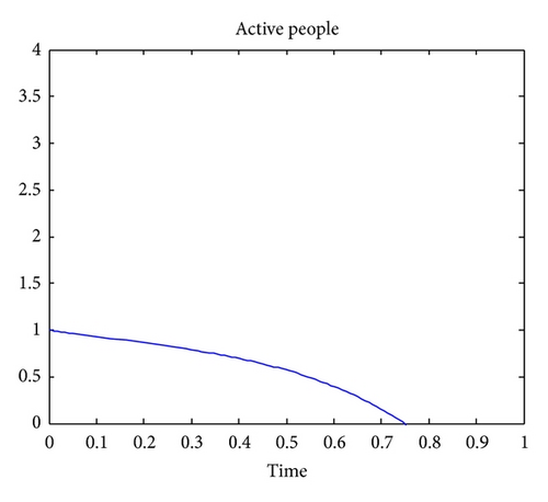
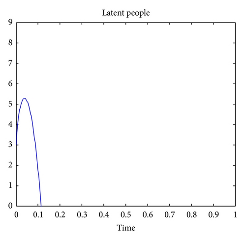
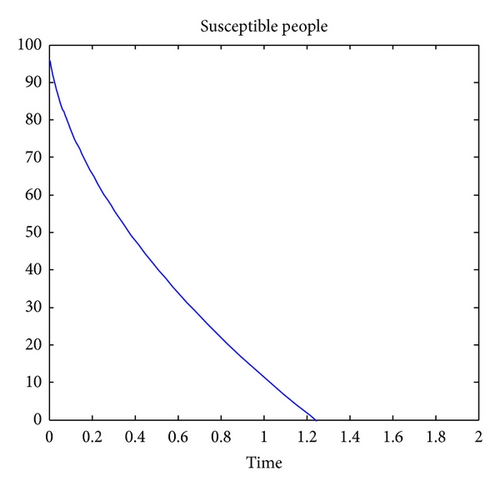
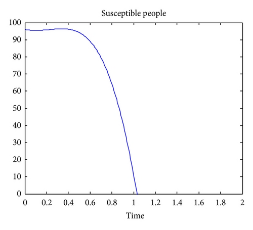
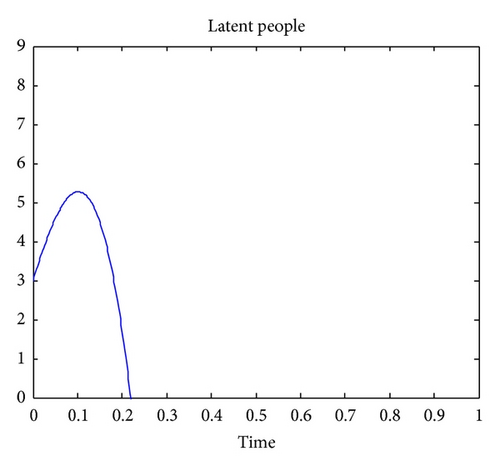
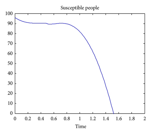
If in addition we assume that no new person migrates or is born in this area, we obtain the following figures. The approximate solutions of the main problem are depicted in Figures 1, 2, and 3, respectively.

Details are in the caption following the image — **Figure 1**
Open in figure viewer PowerPoint

Approximate solution for the number of susceptible people in the location.

Figure 1 shows that, if there is migration or newborn in the location of interest, the number of susceptible people will vanish as time goes, because of the natural death rate and due to TB. Note that any person that is latently infected is removed from the set of susceptible. Figure 2 indicates that the number of people that are latently infected will increase up to a certain time and then vanish as time goes. The number of susceptible people, will become latently infected since some are not vaccinated against the TB and finally will vanish due to. Figure 3 indicates that the number of TB actively infected people will also vanish because of the natural death rate and the death due to TB.

4. Application of the HDM to the Model with Noninteger-Order Derivative

Fractional calculus has been used to model physical and engineering processes, which are found to be best described by fractional differential equations. It is worth noting that the standard mathematical models of integer-order derivatives, including nonlinear models, do not work adequately in many cases. In the recent years, fractional calculus has played a very important role in various fields such as mechanics, electricity, chemistry, biology, economics, notably control theory, and signal and image processing. Major topics include anomalous diffusion; vibration and control; continuous time random walk; Levy statistics, fractional Brownian motion; fractional neutron point kinetic model; power law; Riesz potential; fractional derivative and fractals; computational fractional derivative equations; nonlocal phenomena; history-dependent process; porous media; fractional filters; biomedical engineering; fractional phase-locked loops, and groundwater problem (see [14–21]).

4.1. Properties and Definitions

Definition 1. A real function f(x), x > 0, is said to be in the space C_μ, μ ∈ ℝ, if there exists a real number p > μ, such that f(x) = x^ph(x), where h(x) ∈ C [0, ∞), and it is said to be in space if f^(m) ∈ C_μ, m ∈ ℕ.

Definition 2. The Riemann-Liouville fractional integral operator of order α ≥ 0, of a function f ∈ C_μ, μ ≥ −1, is defined as

()

Properties of the operator can be found in [14–16]. We mention only the following: for f ∈ C_μ, μ ≥ −1, α, β ≥ 0, and γ > −1,

()

Lemma 3. If m − 1 < α ≤ m, m ∈ ℕ, and , μ ≥ −1, then

()

Definition 4 (partial derivatives of fractional order). Assume now that f(x) is a function of n variables x_i i = 1, …, n also of class C on D ∈ ℝ_n. We define partial derivative of order α for f respect to x_i the function

()

where

is the usual partial derivative of integer-order m.

4.2. Approximate Solution of Fractional Version

The system of equations under investigation here is given as

()

Following the discussion presented earlier, we arrive at the following equations:

()

Integrating the previous, we obtain the following components:

()

The remaining terms can be obtained in the same manner. But here only few terms of the series solutions are considered, and the asymptotic solution is given as

()

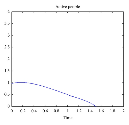
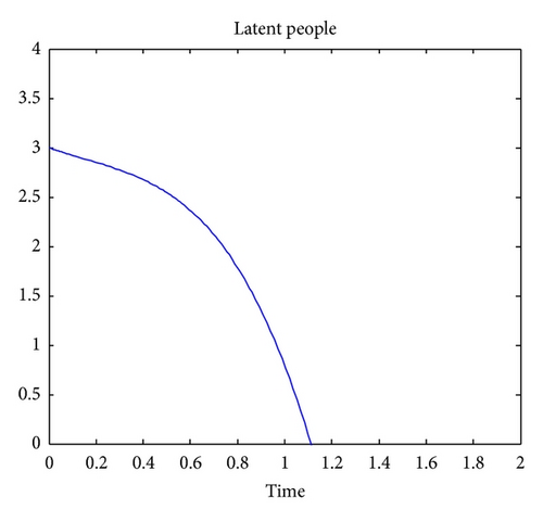
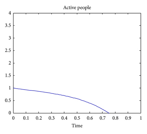
The following figures show the simulated solutions for different values of the fractional order derivatives. The approximate solutions of the main problem are depicted in Figures 4, 5, 6, 7, 8, and 9, respectively.

The numerical simulations show that the approximate solutions are continuous functions of the noninteger-order derivative. It is worth noting that the standard mathematical models of integer-order derivatives, including nonlinear models, do not work adequately in many cases. It is therefore advisable to use the fractional model for describing this problem.

5. Conclusion

The tuberculosis model was examined for the case of integer- and noninteger-order derivatives. Both systems of nonlinear equations were solved with an iterative analytical model called the homotopy decomposition model method. The basic characters of the relatively new technique are presented in detail. The approximate solutions of the noninteger case are increasing continuous functions of the fractional order derivative. The technique used for solving these problems is friendly, very easy, and less time consuming. The numerical solutions in both cases display the biological behaviour of the real world situation.

References

1 Kumar V., Abbas A. K., Fausto N., and Mitchell R. N., Robbins Basic Pathology, 2007, 8th edition, Saunders Elsevier.
Google Scholar
2 Konstantinos A., Testing For Tuberculosis, 2010, 33, Australian Prescriber.
Google Scholar
3 Castro K. G., Global tuberculosis challenges, Emerging Infectious Disease. (1998) 4, no. 3, 408–409.
10.3201/eid0403.980316
CAS PubMed Web of Science® Google Scholar
4 Dye C., Fengzengb Z., Scheele S. et al., Evaluating the impact of tuberculosis control number of deathsprevented by short-course chemotherapy in China, International Journal of Epidemiology. (2000) 29, no. 3, 558–564, https://doi.org/10.1093/ije/29.3.558.
10.1093/ije/29.3.558
CAS PubMed Web of Science® Google Scholar
5 Gammaitoni L. and Nucci M. C., Using a mathematical model to evaluate the efficacy of TB control measures, Emerging Infectious Diseases. (1997) 3, no. 3, 335–342.
10.3201/eid0303.970310
CAS PubMed Web of Science® Google Scholar
6 Murray C. J. and Salomon J. A., Using Mathematical Models To Evaluate Global Tuberculosis Control Strategies—A Paper Presented at the Centre For Population and Development Studies, 1998, Harvard University, Cambridge, Mass, USA.
Google Scholar
7 World health Organization, WHO: Tuberculosis Fact Sheet, 2007.
Google Scholar
8 Koriko O. K. and Yusuf T. T., Mathematical model to simulate tuberculosis disease population dynamics, American Journal of Applied Sciences. (2008) 5, no. 4, 301–306, https://doi.org/10.3844/ajassp.2008.301.306.
10.3844/ajassp.2008.301.306
Google Scholar
9 Baleanu D., Diethelm K., Scalas E., and Trujillo J. J., Fractional Calculus Models and Numerical Methods Series on Complexity, Nonlinearity and Chaos, 2012, World Scientific.
10.1142/8180
Google Scholar
10 Atangana A., Ahmed A., and Belic N., A generalized version of a low velocity impact between a rigid sphere and a transversely isotropic strain-hardening plate supported by a rigid substrate using the concept of non-integer derivatives, Abstract Applied Analysis. (2013) 2013, 9, 671321, https://doi.org/10.1155/2013/671321.
10.1155/2013/671321
Google Scholar
11 Atangana A. and Botha J. F., Analytical solution of the groundwater flow equation obtained via homotopy decomposition method, Journal of Earth Science & Climatic Change. (2012) 3, https://doi.org/10.4172/2157-7617.1000115.
10.4172/2157-7617.1000115
Google Scholar
12 Atangana A. and Alabaraoye E., Solving a system of fractional partial differential equations arising in the model of HIV infection of CD4⁺ cells and attractor one-dimensional Keller-Segel equations, Advances in Difference Equations. (2013) 2013.
10.1186/1687-1847-2013-94
PubMed Google Scholar
13 Atangana A. and Secer A., Time-fractional coupled- the korteweg-de vries equations, Abstract Applied Analysis. (2013) 2013, 8, 947986, https://doi.org/10.1155/2013/947986.
10.1155/2013/947986
Google Scholar
14 Oldham K. B. and Spanier J., The Fractional Calculus, 1974, Academic Press, New York, NY, USA, MR0361633, ZBL0292.26011.
Google Scholar
15 Podlubny I., Fractional Differential Equations, 1999, Academic Press, New York, NY, USA, MR1658022, ZBL1056.93542.
Web of Science® Google Scholar
16 Kilbas A. A., Srivastava H. M., and Trujillo J. J., Theory and Applications of Fractional Differential Equations, 2006, Elsevier Science B.V., Amsterdam, The Netherlands, MR2218073, https://doi.org/10.1016/S0304-0208(06)80001-0, ZBL1206.26007.
10.1016/S0304-0208(06)80001-0
Google Scholar
17 Atangana A. and Secer A., A note on fractional order derivatives and Table of fractional derivative of some specials functions, Abstract Applied Analysis. (2013) 2013, 279681, https://doi.org/10.1155/2013/279681.
10.1155/2013/279681
Google Scholar
18 Caputo M., Linear models of dissipation whose Q is almost frequency independent, part II, Geophysical Journal International. (1967) 13, no. 5, 529–539, https://doi.org/10.1111/j.1365-246X.1967.tb02303.x.
10.1111/j.1365-246X.1967.tb02303.x
Web of Science® Google Scholar
19 Samko S. G., Kilbas A. A., and Marichev O. I., Fractional Integrals and Derivatives: Theory and Applications, 1993, Gordon and Breach, Yverdon, Switzerland, MR1347689, ZBL0924.44003.
Google Scholar
20 Baleanu D., Diethelm K., Scalas E., and Trujillo J. J., Fractional Calculus, 2012, World Scientific, Series on Complexity, Nonlinearity and Chaos, Models and numerical methodshttps://doi.org/10.1142/9789814355216, MR2894576, ZBL1258.35201.
10.1142/8180
Google Scholar
21 Atangana A. and Kılıçman A., A possible generalization of acoustic wave equation using the concept of perturbed derivative order, Mathematical Problems in Engineering. (2013) 2013, 6, 696597, https://doi.org/10.1155/2013/696597.
10.1155/2013/696597
Web of Science® Google Scholar

Citing Literature

All articles

Approximate Solution of Tuberculosis Disease Population Dynamics Model

Abstract

1. Introduction

2. Fundamental Information about Homotopy Decomposition Method

3. Application of the HDM to the Model with Integer-Order Derivative

4. Application of the HDM to the Model with Noninteger-Order Derivative

4.1. Properties and Definitions

4.2. Approximate Solution of Fractional Version

5. Conclusion

References

Citing Literature

Figures

References

Information

About Wiley Online Library

Help & Support

Opportunities

Connect with Wiley

Approximate Solution of Tuberculosis Disease Population Dynamics Model

Abstract

1. Introduction

2. Fundamental Information about Homotopy Decomposition Method

3. Application of the HDM to the Model with Integer-Order Derivative

4. Application of the HDM to the Model with Noninteger-Order Derivative

4.1. Properties and Definitions

4.2. Approximate Solution of Fractional Version

5. Conclusion

References

Citing Literature

Figures

References

Related

Information