Today’s standard robotic systems often do not meet the industry’s demands for accurate high-speed robotic applications. Any machine, be it an existing or a new one, should be pushed to its limits to provide “optimal” efficiency. However, due to the high complexity of modern applications, a one-step overall optimization is not possible. Therefore, this contribution introduces a step-by-step sequence of multiple nonlinear optimizations. Included are optimal configurations for geometric calibration, best-exciting trajectories for parameter identification, model-based control, and time/energy optimal trajectory planning for continuous path and point-to-point trajectories. Each of these optimizations contributes to the improvement of the overall system. Existing optimization techniques are adapted and extended for use with a standard industrial robot scenario and combined with a comprehensive toolkit with discussions on the interplay between the separate components. Most importantly, all procedures are evaluated in practical experiments on a standard robot with industrial control hardware and the recorded measurements are presented, a step often missing in publications in this area.

1. Introduction

State-of-the-art robotic systems are equipped with highly sophisticated industrial hardware, capable of short sample times and offering high computational power. This increasing arithmetic performance may be used to improve positioning accuracy and dynamic accuracy and compute time/energy-optimal trajectories. The proper fundamentals are found in the underlying mathematical models.

This contribution focuses on giving an overview of various nonlinear optimizations. With each optimization, a certain aspect of an arbitrary robotic system is improved. Applying all of them in sequence will provide better results regarding positioning accuracy and dynamic accuracy and will reduce the cycle times. The basis for this optimization lies in the kinematic and dynamical modeling of the system. Therefore, Section 2 starts with the deviation of these models enhanced by a model-based control strategy. Special emphasis is laid on the implementation on an industrial system including time delays. In Section 3, the static position accuracy of the robot is improved by considering unavoidable tolerances in the robot kinematics. The main topic is obtaining optimal configurations for the identification process. The identification of the dynamic parameters, that are used for the model-based control, is described in Section 4. Also, the problem of optimal exciting trajectories is solved by nonlinear optimization techniques. Finally, Section 5 reviews time/energy optimal trajectory planning for continuous path trajectories and point-to-point trajectories.

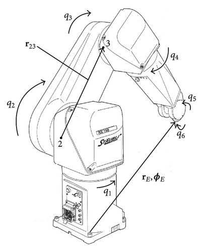
Each section provides information on the used solvers for the various optimizations and also presents detailed results of the conducted experiments. Experiments are performed using an off-the-shelf robot, a Stäubli RX130L shown in Figure 3, with industrial control hardware and commercially available measurement hardware, to guarantee that all proposed methods are applicable for industry. For specifications of the articulated robot, please consult Table 1.

Table 1. Technical specifications.

Stäubli RX130L industrial robot
Degrees of freedom	6
Maximum load capacity	10 kg
Reach at wrist	1660 mm
Weight	≈200 kg

Previous works of the authors, which are also focused on industrial robotics, see, for example, [1], cover the basics like control and geometric path planning. Based on these works, a specific combination of algorithms is presented, each of which optimizes a specific aspect of the robotic system.

2. System Modeling and Control

2.1. Kinematic Modeling

The kinematic modeling can be divided in the direct kinematics problem and the inverse kinematics problem. The direct kinematics calculates the end-effector coordinates

as a function of the joint coordinates q and nominal geometric parameters p_n as

(1)

see Figure 3. Vector r_E indicates the end-effector position, which can be calculated by a sequential summation of the relative connecting vectors. For the orientation, a description in Cardan angles is used. A sequential multiplication of the relative rotation matrices between two successive joints delivers the rotation matrix A_IE between end-effector frame (E) and inertial frame (I) from which the Cardan angles can be extracted. In this paper, also the notation tool center point (TCP) is used for the end-effector. Inverse kinematics calculates the joint coordinates q as a function of end-effector coordinates z_E and p_n:

(2)

Solutions for the inverse kinematics problem of such standard robotic systems can be found in many textbooks, for example, [2] or [3].

2.2. Dynamic Modeling

The equations of motion for multibody systems, like a robot, can be calculated by several methods. The method with minimal effort is the Projection Equation, see [4]. Linear momenta p = mv_c and angular momenta L = Jω_c are projected into the minimal space (minimal velocities

) via the appropriate Jacobian matrices:

(3)

All the values like the translational velocity v_c or the rotational velocity of the center of gravity ω_c can be inserted in arbitrary coordinate systems R. In contrast to ω_c, ω_IR is the velocity of the used reference system. The matrix J is the inertia tensor, while

characterizes the vector product ω × p. f^e and M^e are impressed forces and moments acting on the ith body. An evaluation of (3) yields the highly nonlinear equations of motion for the robot

(4)

They are composed of the minimal coordinates q, the configuration dependent, symmetric and positive definite mass matrix M(q), the vector

containing all nonlinear effects (like Coriolis, centrifugal, gravity, and friction forces), and the vector of the generalized actuating forces Q_M.

Detailed dynamical modeling is an essential task because it is the basis for model-based control and optimal trajectory generation.

2.3. Control

The hardware setup is composed of an industrial PC, communicating via Powerlink with six ACOPOS servo drives, which power the synchronous motors of the Stäubli robot. The servo drives use cascaded controllers for precise position control of the robot’s joints. However, the articulated robot is a highly nonlinear system due to the serially connected arm/joint units. Typically, using linear joint controllers on a highly nonlinear mechanical system will not lead to sufficiently accurate and dynamic end-effector motion.

2.3.1. Model-Based Control

This contribution suggests to effectively linearize the nonlinear mechanical system with a flatness-based feed-forward approach and use the servo drives’ linear cascaded controllers to compensate model deviations and external disturbances. Thus, they are summarized for the sake of completeness. Introducing the state

, the equations of motion, (4), in state space read

(5)

with the input vector of motor torques Q_M. With the flat output y = q and its derivatives with respect to time,

(6)

all state and input variables can be computed as a function of the flat output, see, for example, [5]. Consequently, the evolution of all system variables q,

, and Q_M is determined by a sufficiently smooth trajectory y(t).

Thus, combining the superimposed feed-forward branch with the servo drives’ internal controllers yields the control law for the motor torques Q_M:

(7)

Please note that the feed-forward term in (7) guides the system states along the desired trajectory, while the feed-back control law ensures stability against disturbances and modeling errors with the positive diagonal matrices K_p and K_d. The stability of the overall system, applying (7), is proven in [6]. Alternatively, the feed forward control law may also be computed by using the structural properties of the robot’s subsystem representation, as described in [7].

2.3.2. Implementation

In order to evaluate the quality of the suggested controls, the Stäubli RX130L robot is interfaced with the motion hardware. During this process, the robot’s mechanics, AC motors, and resolvers are not changed or manipulated in any way.

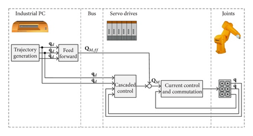
The industrial PC is using 400 μs as base sample time. Every sample step, the inverse kinematic problem is solved numerically to transform the desired end-effector movement into corresponding joint positions, velocities, and accelerations. With these reference joint variables (, and ), the mathematical model is evaluated to compute the feed-forward motor torques as stated in (7). Then, for each joint, a separate Ethernet telegram is generated containing the reference positions and corresponding feed-forward motor torques.

The servo drives are parameterized to accept cyclic position inputs for the cascaded controller. To do so, the cyclically arriving network telegrams are received and the desired reference positions are passed to the set value inputs of the cascaded controllers. Also, the computed feed-forward torques are transformed to corresponding motor currents and added to the servo drives’ current controllers set values. Figure 1 presents the corresponding block diagram.

Details are in the caption following the image — **Figure 1**
Open in figure viewer PowerPoint

Block diagram of the control structure.

2.3.3. Experimental Results

The quality of the implemented control strategy is validated by experiments with the Stäubli RX130L robot. Regarding industrial interests, the standardized trajectory found in the EN ISO NORM 9283, see [8], is used as reference trajectory. It consists of various elements: circles, straight lines, and squares in the typical workspace for an industrial application. The TCP velocity is chosen with 1 m/s and its acceleration with 5 m/s².

Figure 2(a) depicts the the lag errors of the first three joints. The other axes show similar results. The positive influence of the feed-forward loop is clearly observable. To present insights on the TCP-accuracy during high dynamics, the TCP errors for the standard and the improved control law along the trajectory are presented in Figure 2(b). They are measured using a high-precision laser tracker LTD600 from Leica at a sampling rate of 1 ms.

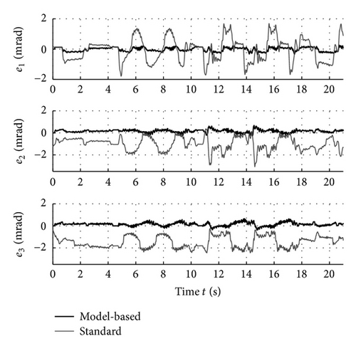
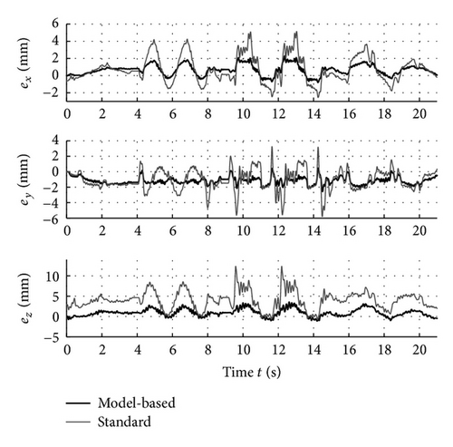
Obviously, the positive effects of the model-based feed-forward approach drastically reduce the TCP and joint errors. Mainly, they compensate static effects, for example, resulting from gravity, and dynamic effects, for example, arising from friction and high accelerations while the standard cascaded controller provides stiffness, stability, and robustness.

3. Static Position Accuracy

Industrial robotic systems usually offer a satisfying repeatability. However, the lack of sufficient accuracy of the end-effector is responsible for time-consuming adjustments while commissioning new tasks. The sources of these errors are nonmodeled manufacturing tolerances, assembly inaccuracies, and joint encoder offsets.

3.1. Kinematics with Error Parameters

The direct kinematics, which compute the end-effector position r_E and orientation φ_E as function of the joint angles q and nominal geometric parameters p_n, can be extended by a set of error parameters p_e regarding lengths, joint offsets, and assembly inaccuracies. For example, the connection vector between points 2 and 3 reads

(8)

where l₂ is the nominal length of the connection (part of p_n) and p_e2x, p_e2y, p_e2z are the position error values (part of p_e). Thus, the robot’s TCP position and orientation is

(9)

For a standard six-axis industrial robot, as sketched in Figure 3, p_e contains 6 · 3 error parameters regarding length, 6 joint encoder offsets, 6 · 2 angles for misaligned coordinate frames between each link, and 3 tolerances for defining the inertial coordinate system. This results in a set of 39 parameters. To remove all linear dependencies, a QR-decomposition is applied, see Section 4.1 for details. Applying this method yields the final error parameter p_e ∈ ℝ³⁰.

3.2. Geometric Calibration

The calibration process calculates valid values for the error parameter p_e that minimize the error e between measured TCP-positions z_M and TCP-positions determined using the corresponding joint angles q:

(10)

This highly nonlinear equation can be solved by an iterative method. Representing (10) as a Taylor-series around p_e, neglecting higher order terms and demanding that the error converges towards zero, yields

(11)

For m measurements, (11) becomes

(12)

which is an overdetermined equation system solvable by standard least-squares techniques. The minimum of the quadratic error is found with

(13)

yielding the update law for the error parameter vector

(14)

Initial values for

can be assumed to be zero because the error parameters regarding length, and so forth, are considerably smaller than the nominal geometric parameters. To finally obtain good position accuracy, the identified parameters p_e must be considered in the inverse kinematics algorithm. Any suitable numerical solution is viable and can handle the set of additional parameters.

3.3. Optimal Configurations for Calibration

It is obvious that the geometric calibration only identifies parameters well that are excited accordingly. To overcome this problem, the whole work- or joint-space could be discretized for taking the necessary measurements. While this approach is viable for small systems, it is heavily time and cost consuming for systems with multiple degrees of freedom. Such complex systems are common in today’s industrial applications. As a consequence, an optimal set of configurations, which guarantees well-excited error parameters, needs to be found.

3.3.1. Observation Index and Algorithm

In order to ensure a well-conditioned problem formulation and also well-excited parameters p_e, the minimum singular value of the covariance matrix Λ = Θ^TΘ in (14) is used as observation index and optimization criterion and further described by B = σ_m(Λ). As, for example, [9–11] show, there exist various choices for valid observation indices with slightly different properties. The proposed algorithm, which has been presented in [12], allows the use of arbitrary observation indices.

Before introducing the optimization algorithm, two basic operations are defined:

(i)
Add a configuration: adding a new configuration with the Jacobian to the current information matrix Θ_i yields
(15)
which directly influences the change of the chosen observation index
(16)
(ii)
Remove a configuration: similar to the previous case, removing a configuration from the current information matrix Θ_i is described by
(17)

Additionally, the complete set of N measurable configurations is called the configuration-set Π. An arbitrary subset of it is denoted by the set ξ. These operations and definitions are the basics for the following optimization method.

(1)
Initialization: a given number of n configurations is randomly selected from the initial configuration-set Π. This subset ξ₀ must lead to a nonsingular covariance-matrix Λ₀ to ensure a computation of the observation index B(Λ₀). Should this not be the case for the chosen configurations, then the random selection process is simply repeated.
(2)
Remove and replace: the configuration that leads to the minimal decrease of the observation index, ΔB(Λ_i+1), is removed from the current configuration set ξ_i. Then, the resulting subset ξ_i+1 is complemented by exactly that configuration of Π that maximizes ΔB(Λ_i+2). For both operations, the correct element is found by an exhaustive search over the respective set. Note that due to the simple way to calculate ΔB (see ((15)–(17))), the computational effort for these searches is not as dramatic as it may sound. This remove-and-replace strategy effectively sorts out configurations that do not improve the overall conditioning of the covariance matrix and replaces them with ones that do. The step is repeated as long as one remove-and-replace operation still improves the observation index. Otherwise, the next step is executed.
(3)
Add additional configurations: from the configuration-set Π exactly the one configuration (again, found by exhaustive search) that, by itself, maximizes ΔB(Λ_i+i), is added to the current subset ξ_i. This step is iterated until the observation index cannot be further increased by such an operation or until a user-specified maximum number of desired configurations is reached. Otherwise, execute the final step.
(4)
Final remove and replace: analogously to step 2, each single configuration of the subset ξ_i is evaluated. If any remove and replace operation as described above still increases the observation index, this exchange is executed. Otherwise, the procedure is terminated.

The algorithm may be applied multiple times to prevent getting stuck at a local minimum. The solution with the maximum observation index is used for the experimental analysis. Nevertheless, finding these optimal configurations is time consuming and lasts about five minutes on a standard PC. Since these calculations are performed offline before any measurements are done, this is not a critical issue.

3.4. Experimental Results

To evaluate the performance of the proposed algorithm, detailed experimental results for the RX130L robot are presented. First, the robot’s joint-space is discretized by 13 equally large intervals per degree of freedom. This results in a set of 13⁶ ≈ 4.8 · 10⁶ configurations. In reality the coordinates of the end-effector are measured by the visual infrared tracker system 3D-Creator, manufactured by the Boulder Innovation Group. A probe emitting infrared light by 4 diodes is mounted on the end-effector of the robot. This light is recorded by three CCD cameras and the position and orientation in world coordinates are calculated by stereovision. Robot configurations that are not visible by this system are removed. The remaining set consists of approximately 4000 configurations. Then, the algorithm is used to compute 32 optimal configurations. As Figure 4 emphasizes, the optimal configurations differ strongly from each other to keep the condition number of the covariance matrix low, also leading to well-excited parameters. Compared to a linear scan of the workspace, the observation index is reduced by the factor 18.5 while keeping the number of necessary measurements very small.

For information on the position and orientation accuracy before (uncal., p_e = 0) and after calibration (cal), see Table 2. The orientation errors are represented in Cardan angles.

Table 2. Errors before (uncal., p _e = 0) and after geometric calibration (cal.).

	Position and orientation errors
	Maximum		Peak-to-peak
	uncal.	cal.	uncal.	cal.
e_x in mm	7.779	0.272	±6.171	±0.271
e_y in mm	19.026	0.310	±4.267	±0.303
e_z in mm	12.614	0.414	±1.402	±0.376
e_α in ^∘	1.140	0.128	±0.272	±0.109
e_β in ^∘	1.817	0.191	±0.335	±0.182
e_γ in ^∘	1.160	0.131	±0.514	±0.116

4. System Identification

In this section, the identification of the dynamical parameters describing the robot behavior, see (4), is covered. This is clearly an essential task because it is the basis for model-based control and optimal trajectory generation.

4.1. Dynamic Parameter Identification

An important property of the equations of motion is the linearity with respect to dynamic parameters p ∈ ℝ^p characterizing the robot links and motors. By introducing the information matrix Θ ∈ ℝ^n,p (n degrees of freedom), (4) can be restructured to

(18)

The parameter vector p is the composition of the the joint parameters p_joint,i

(19)

containing the mass m_i, the center of mass r_c,i, the elements of the inertia tensor

, and Coulomb/viscous friction coefficients d_c,i and d_v,i for the ith joint-arm unit. Since the dynamical parameters are confidential manufacturer data, all these parameters have to be identified. Usually, the information matrix Θ and the parameter vector p contain linear dependencies, which have to be removed before the identification process. A QR decomposition and reformulation leads to

(20)

where

is an orthogonal matrix and

is an upper triangular matrix. The nonidentifiable parameters are those whose corresponding elements on the diagonal of the matrix

are zero. In contrast, if

, then the corresponding column in Θ is independent. Let the p − s independent columns be collected in the matrix Θ₁ and the corresponding parameters be collected in p₁. The dependent columns and parameters are represented by Θ₂ and p₂, respectively, such that

(21)

is fulfilled, since Θ₂ is linearly dependent on Θ₁ by a matrix κ ∈ ℝ^p−s,s. In (21) κ can be shifted to the parameters leading to

(22)

with the base parameters p_b ∈ ℝ^p−s. For the calculation of κ, (20) is again evaluated with separated matrices [Θ₁Θ₂] and

, respectively, yielding

(23)

and therefore

(24)

Combining (23) and (24), κ can be obtained as

(25)

It contains geometric parameters like lengths, lengths squared, gear ratios, and so on, see [13] for details. The identification process can be performed by sequentially arranging k ≫ p − s measurements in (18) and (22) leading to

(26)

The unknown base parameters p_b are calculated with the least-squares method leading to

(27)

and therefore the solution

(28)

is directly available since Rank(Θ_f) = p − s.

4.2. Optimal Exciting Trajectories

Similar to the problem of finding optimal configurations for the geometric calibration, the dynamic parameter identification requires exciting trajectories. In contrast to the steady-state configurations for the calibration, the identification trajectories include an additional dimension, the continuous time. Again, the aim is to minimize the condition number (cond) of the covariance matrix by choosing suitable trajectories. A promising approach is introduced with [14]. This section summarizes these ideas, presents solutions to the optimization problem, and verifies the results on the RX130L robot.

4.2.1. Trajectory Description and Optimization

An adequate description for the identification trajectory for the ith joint is given with

(29)

This Fourier-series is parameterized by the finite order N_i, the coefficients a_i,l and b_i,l, the base angular frequency ω_f, and the joint offset q_i0. To guarantee a periodic excitation of the robot, ω_f is a common parameter for all joints. To speed up the optimization time, a discretization of (29) and derivatives for one period of the base frequency (T_f = 2π/ω_f) is done. The signals are therefore evaluated at discrete time values iΔT, i = 0 ⋯ k, ΔT = T_f/k, where k is the number of discretization points. This provides the following optimization problem:

(30)

The constraints include the mechanical joint limits q_max, the permitted joint velocities

, the expected maximum joint accelerations

, and a space of allowed end-effector positions

, which is used to avoid collisions with the robot itself and its surroundings. Due to the flatness property of the system, see Section 2.3.1, also the motor torques can be calculated dependent on the joint coordinates and derivatives. In contrast to [15], this motor torques are also used in our formulation. The optimization problem is solved with the Matlab-Optimization-Toolbox (fmincon). The parameters order N = 5, angular frequency ω_f = 0.8 rad/s, and k = 80 turned out to work well to get adequate dynamical parameters, see Figure 5(b). For numerical scaling purposes, the columns of Θ_f should also be normalized. Solving the optimization problem yields the optimal joint trajectories.

4.3. Experimental Results

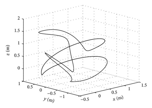
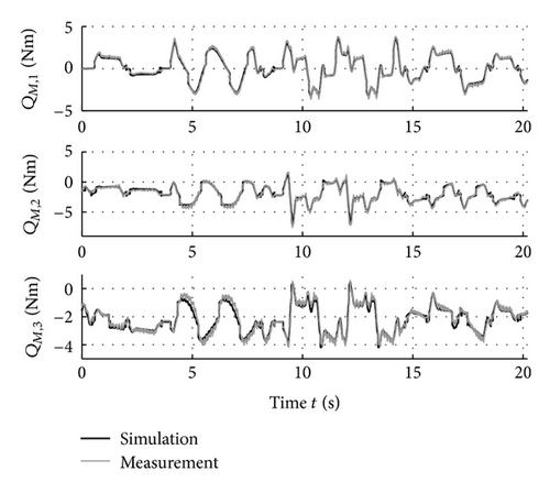
The measurements for the overdetermined equations system (28) are taken to estimate the dynamical base parameters p_b. Figure 5(a) presents a plot of the end-effector path. Along the path, velocities up to 5 m/s and accelerations up to 12 m/s² are achieved. To verify the quality of the identified parameters, the real robot’s motor torques are recorded and compared to the simulated ones on a reference trajectory which is defined in the EN ISO NORM 9283, see [8]. Figure 5(b) emphasizes, by presenting the measured and simulated motor torques, the good parameter identification for the RX130L robot. Joints four, five, and six show an equivalent quality.

5. Optimal Trajectory Generation

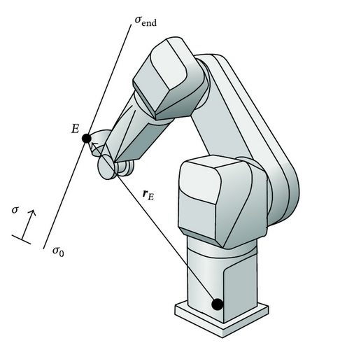
There are two types of trajectory generation problems that have to be considered. The first one is the continuous path (CP) trajectory and the second one is the point-to-point (PtP) trajectory planning problem. For the first one, the geometric path in world coordinates is defined. Typical maneuvers are straight lines, circles, and splines. For the PtP planning, only the coordinates for the start-point z_E,0 and the end-point z_E,end of the trajectory are given. These points can directly be transformed to joint coordinates q₀, q_end, and the motion planning can be performed in this coordinates. For both cases, physical constraints like motor speeds and torques have to be taken into account. Additionally, the computed trajectories have to result in continuous velocities, accelerations, and jerks. This helps that the gear elasticities are not overly excited, leading to a soft, vibration-less end-effector movement. Again, the equations of motion, derived in Section 2.2 and identified in Section 4, provide the basis for this approach.

5.1. Continuous Path Trajectory

CP applications appear in many robotic applications like arc welding, deburring, and laser cutting. Due to the nonlinear kinematic interrelation between Cartesian space and the robot’s joint space, high motor speeds and accelerations may occur, especially near kinematic singularities. The CP motion planning can be divided into two subproblems, namely, a geometric path planner, describing a path z_E(σ)

(31)

as a function of a (scalar) trajectory parameter σ ∈ [σ₀, σ_end] and a dynamic path planner that solves the problem of finding an optimized time behavior σ(t), see also [16]. For example, a straight line in space is characterized by (39). The vector r_E contains the end-effector position while φ_E describes the evolution of the orientation in Cardan angles, both are functions of σ. The trajectory parameter σ itself is a function of time σ = σ(t) and the corresponding trajectory velocity and acceleration are

(32)

The trajectory parameter and its derivatives (trajectory speed and acceleration) represent the trajectory and its evolution in a demonstrative and easily interpretable manner. Figure 6 shows an example for a straight line, beginning at σ₀ and ending at σ_end. With six degrees of freedom and six world coordinates, the analytical solution of the inverse kinematic problem, see for example, [3], for the RX130 robot is obtained

(33)

which can be differentiated with respect to time, leading to

(34)

Inserting the kinematic relations (33) and (34) into the equations of motion (4) yields the following description of the robot’s dynamics:

(35)

This representation allows to compute the motor torques as a function of the trajectory position, velocity, and acceleration. For additional details, see [17]. Please note that the inverse kinematics does not necessarily have to be computed analytically. Also numerical calculations of the inverse kinematics can be used.

5.2. Optimization Strategy

To find an optimal evolution along a desired trajectory, the objective reads

(36)

where the motor torques Q_M are calculated in (35). The design parameters k₁ and k₂ are manipulated to weight between time and/or energy optimality. However, the upper limit of the integral in (36) is unknown in advance, merely a result of optimization.

Thus, a transformation with

leads to an objective function with constant integration limits and σ as integration variable. Equation (38) summarizes the result. The objective function is also subject to a set of differential equations, describing the evolution of time along the trajectory parameter σ. The derivatives with respect to σ are used to compute all trajectory variables, which are found in the constraints. For instance, the trajectory acceleration is computed with

(37)

where a prime indicates the differential operator (·) ^′ = d(·)/dσ. The input u in the set of differential equations needs to be computed by a numerical solver in order to minimize the objective function while satisfying all constraints.

Finalizing the following complete description:

(38)

the motor torques, motor velocities, and accelerations are constrained. To compute an optimal solution u for the optimization problem stated in (38), the MUSCOD-II software package is utilized. Based on [18], it is developed by the Interdisciplinary Center for Scientific Computing at the University of Heidelberg. Using the direct multiple-shooting method, see [19, 20], the original continuous optimal control problem is reformulated as a nonlinear programming (NLP) problem which is then solved by an iterative solution procedure, a specially tailored sequential quadratic programming (SQP) algorithm. For further details on the used software package, see [21].

5.3. Experimental Results—CP Trajectory

For a straight tool center movement with constant end-effector orientation, the trajectory is given by

(39)

where index 0 indicates the start-point and index end the end-point, respectively. For a grid of 200 shooting intervals, the time optimal case k₁ = 1, k₂ = 0 is computed. Minimizing energy would lead to not only smoother, but also longer trajectories for σ and is therefore not considered in this example. The resulting trajectory parameters

, and

are retransformed into the time domain to compute the corresponding reference joint angles q_d(t) and the constrained feed-forward torques Q_M,ff(t). The corresponding velocity profile is depicted in Figure 7. The velocity-drop occurs due to passing closely to a singular configuration.

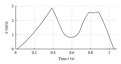
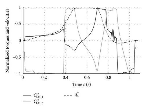
The experiment with the Stäubli robot is conducted analogously to the previous section. The reference angles and torques are transferred to the servo drives where the occurring torques and motor velocities are measured for verification. Figure 8 shows the torques and velocities of the axes that actively constrain the trajectory. For readability reasons, the signals are normalized to their maximum values. The figure also shows that at least one constraint is always active, which is a necessary condition for the time-optimal solution.

5.4. Point-to-Point Trajectory

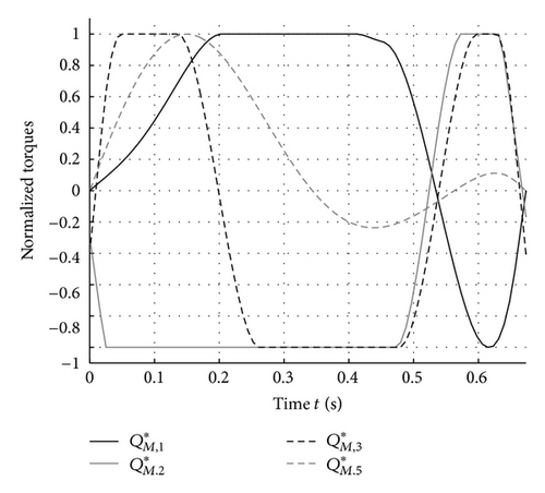
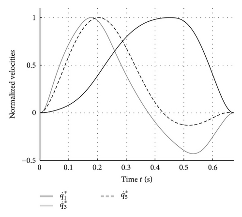
As an extension to the previous section, the PtP optimization is not limited to geometrically defined paths. Consequently, the one-dimensional variation of the trajectory parameter becomes a more complex two-point boundary value problem of the joint states with the additional task of minimizing time and/or energy, summarized in (40). Analogously to (38), the available joint velocities and torques are limited. Additionally, the joint limits q_max need to be considered and the desired initial and final configurations q₀, , q_e, and are introduced.

A compromise between time and energy optimality is adjusted with the parameters k₁ and k₂. Also note that the highly nonlinear differential equations of motion are included in the set of constraints.

5.5. Experimental Results—PtP Trajectory

The optimization formulation for the point-to-point trajectory

(40)

is solved with MUSCOD-II setting k₁ = 1 and k₂ = 0 (time optimality). While the one-dimensional variation problem of the previous section is computed in one second, the PtP trajectory takes about three minutes to be calculated with a standard workstation. After solving the optimization problem, the system states and torque inputs for the two-point boundary problem are known and may be utilized as reference values. The initial conditions q₀,

, q_e, and

are chosen equals to the start- and endpoint of the previous section’s straight-line trajectory. This allows a comparison between both methods. The overall time of the trajectory was reduced from t_e = 1.04 s to t_e = 0.67 s. Figures 9(a) and 9(b) show the optimized torques and velocities. Again, the most interesting signals are selected for reasons of readability, all normalized to their maximum values. Experiments using these results on the RX130L robot verify validity of the optimized trajectory. The maximum end-effector velocity and acceleration that are reached along this trajectory are 5.2 m/s and 48.6 m/s², respectively. To avoid high jerks in joint space, which would induce vibrations, the torque rates are limited to

6. Conclusions

This work summarizes various optimization strategies for robotic systems to improve the overall performance. The individual results of each section not only verify the chosen approach but also offer values for expected accuracies of modern medium scale robotic systems. The suggested ideas are also applicable to smaller or larger scale robots with an arbitrary amount of degrees of freedom.

It is important to note that the quality of the control as well as the trajectory optimization is only as good as the underlying set of (kinematic or dynamical) parameters. As a consequence, the optimal configurations for calibration and the optimal-exciting trajectories for the identification process provide the basis for control and trajectory generations. All proposed methods can be automated by designing according to algorithms and used during the commissioning of robot applications.

Acknowledgments

Support of the current work within the framework of the Austrian Center of Competence in Mechatronics (ACCM) is gratefully acknowledged. The support of the Interdisciplinary Center for Scientific Computing at the University of Heidelberg is acknowledged, especially to Moritz Diehl and Andreas Poschka who kindly gave support. One of the basic ideas of this contribution is to review and present details using industrial, not laboratory, equipment. However, the authors do not have a direct relation to any mentioned hardware and software products. This information is consciously included, enabling the reader to review technical specifications for further comparisons.

Supporting Information

References

1 Riepl R. and Gattringer H., Accurate high-speed robotics [Dissertation], 2009, Johannes Kepler University, B&R Industrial Ethernet Award.
Google Scholar
2 Khalil W. and Dombre E., Modeling, Identification and Control of Robots, 2004, Kogan Page Science, London, UK.
Google Scholar
3 Siciliano B., Sciavicco L., Villani L., and Oriolo G., Robotics: Modelling, Planning and Control, 2009, Springer, London, UK, Advanced Textbooks in Control and Signal Processing Series, Edited by A. J. J. Grimble.
Google Scholar
4 Bremer H., Elastic Multibody Dynamics: A Direct Ritz Approach, 2008, Springer, New York, NY, USA.
Google Scholar
5 Isidori A., Nonlinear Control Systems, 1985, Springer, New York, NY, USA.
Google Scholar
6 Kugi A., Introduction to tracking control of finite- and infinite-dimensional systems, Stability, Identification and Control in Nonlinear Structural Dynamics (SICON), 2008.
Google Scholar
7 Gattringer H. and Bremer H., H. Ulbrich and W. G. Günthner, A penalty shooting walking machine, IUTAM Symposium on Vibration Control of NonlInear Mechanisms and Structures, 2005, Springer.
Google Scholar
8 ISO NORM 9283, Manipulating industrial robots—performance and criteria, Norm, EN ISO, 9283, 1998.
Google Scholar
9 Menq C. H., Borm J. H., and Lai J. Z., Identification and observability measure of a basis set of error parameters in robot calibration, Journal of Mechanisms, Transmissions, and Automation in Design. (1989) 111, no. 4, 513–518, 2-s2.0-0024938018.
Google Scholar
10 Driels M. R. and Pathre U. S., Significance of observation strategy on the design of robot calibration experiments, Journal of Robotic Systems. (1990) 7, no. 2, 197–223, https://doi.org/10.1002/rob.4620070206.
Google Scholar
11 Sun Y. and Hollerbach J. M., Observability index selection for robot calibration, Proceedings of the IEEE International Conference on Robotics and Automation (ICRA ′08), May 2008, 831–836, 2-s2.0-51649129870, https://doi.org/10.1109/ROBOT.2008.4543308.
Google Scholar
12 Sun Y. and Hollerbach J. M., Active robot calibration algorithm, Proceedings of the IEEE International Conference on Robotics and Automation (ICRA ′08), May 2008, 1276–1281, 2-s2.0-51749110279, https://doi.org/10.1109/ROBOT.2008.4543379.
Google Scholar
13 Gattringer H., Starr-Elastische Robotersysteme: Theorie und Anwendungen, 2011, Springer, Berlin, Germany.
Google Scholar
14 Swevers J., Ganseman C., De Schutter J., and Van Brussel H., Experimental robot identification using optimised periodic trajectories, Mechanical Systems and Signal Processing. (1996) 10, no. 5, 561–577, 2-s2.0-0030232035, https://doi.org/10.1006/mssp.1996.0039.
Google Scholar
15 Kostić D., de Jager B., Steinbuch M., and Hensen R., Modeling and identification for high-performance robot control: an RRR-robotic arm case study, IEEE Transactions on Control Systems Technology. (2004) 12, no. 6, 904–919, 2-s2.0-7744227603, https://doi.org/10.1109/TCST.2004.833641.
Google Scholar
16 Johanni R., Optimale Bahnplanung bei Industrierobotern, 1988, Technische Universität München, München, Germany.
Google Scholar
17 Riepl R. and Gattringer H., An approach to optimal motion planning for robotic applications, Proceedings of the 9th International Conference on Motion and Vibration Control, 2008.
Google Scholar
18 Leineweber D., Bauer I., Schäfer A., Bock H., and Schlöder J., An efficient multiple shooting based reduced SQP strategy for large-scale dynamic process optimization (Parts I and II), Computers and Chemical Engineering. (2003) 27, 157–174.
Google Scholar
19 Nocedal J. and Wright S. J., Numerical Optimization, 2006, 2nd edition, Springer Science+Business Media, LLC, New York, NY, USA.
Google Scholar
20 Betts J. T., Practical Methods for Optimal Control Using Nonlinear Programming, 2001, Society for Industrial and Applied Mathematics, Philadelphia, Pa, USA.
Google Scholar
21 Diehl M., Leineweber D. B., and Schäfer A., MUSCOD-II Users’ Manual, 2001, Universität Heidelberg, Heidelberg, Germany.
Google Scholar

Citing Literature

All articles

Optimizing Industrial Robots for Accurate High-Speed Applications

Abstract

1. Introduction