We consider the testing problem for the parameter and restricted estimator for the nonparametric component in the additive partially linear errors-in-variables (EV) models under additional restricted condition. We propose a profile Lagrange multiplier test statistic based on modified profile least-squares method and two-stage restricted estimator for the nonparametric component. We derive two important results. One is that, without requiring the undersmoothing of the nonparametric components, the proposed test statistic is proved asymptotically to be a standard chi-square distribution under the null hypothesis and a noncentral chi-square distribution under the alternative hypothesis. These results are the same as the results derived by Wei and Wang (2012) for their adjusted test statistic. But our method does not need an adjustment and is easier to implement especially for the unknown covariance of measurement error. The other is that asymptotic distribution of proposed two-stage restricted estimator of the nonparametric component is asymptotically normal and has an oracle property in the sense that, though the other component is unknown, the estimator performs well as if it was known. Some simulation studies are carried out to illustrate relevant performances with a finite sample. The asymptotic distribution of the restricted corrected-profile least-squares estimator, which has not been considered by Wei and Wang (2012), is also investigated.

1. Introduction

To balance the modeling bias and the “curse of dimensionality,” different kinds of semiparametric models, such as partially linear model, partially linear varying coefficient model, partially linear single-index model, and additive partially linear model, have been proposed and investigated. In this paper, we consider the semiparametric additive partially linear model, which can be written as

()

where Y is the response, X and Z = (Z₁, …, Z_D) ^′ are covariates on R^p and R^D, respectively, f₁, …, f_D are unknown smooth functions, β = (β₁, …, β_p) ^′ is a p-dimensional vector of unknown parameters, and ε is the random error with conditional mean zero given X and Z. Model (1), inheriting the interpretability of the linear model and flexibility of the additive model, has been studied by Opsomer and Ruppert [1], Li [2], and Jiang et al. [3], among others. Two important models, partially linear model, which is the case when D = 1 for model (1), and additive model, when β = 0, can be regarded as its special models.

However in many practical applications, it may be difficult or impossible to measure some explanatory variables accurately, and people usually can only observe its surrogate. For the literature about errors in variables (EV) the reader can resort to Fuller [4], Cheng and Van Ness [5], Carroll et al. [6], Liang et al. [7], You and Chen [8], Li and Greene [9], Wang et al. [10], and the references therein. In this paper, we consider model (1) with the case that only covariate X is measured with additive error; that is, X cannot be observed, but an unbiased measure of X, denoted by W, can be obtained such that

()

where U is the measurement error with mean zero and independent of (X, Z, Y). Like Liang et al. [11], we only consider the case of D = 2 and assume that the covariance matrix of measurement error U, say Σ_uu, is known. Otherwise, we can estimate it by repeatedly measuring W as mentioned by Liang et al. [7, 11].

In many practical applications such as production and consumption studies, in addition to the sample information, people always have some prior information on regression parametric vector which can be formed into some constraint conditions and used to improve the parametric estimators. For more detailed discussion see Jorgenson [12]. It is well known that for general linear models and nonlinear regression models there are restricted estimation and corresponding results, but for semi-parametric regression models, the results of restricted estimation are very few. Recently, Wei and Wang [13] considered the testing problem under the following linear hypothesis on the parametric component:

()

where A is a k × p matrix of known constants, rank (A) = k, and b is a k-vector of known constants. They first proposed the restricted corrected-profile least-squares estimator

of β under the restriction Aβ = b. Based on the difference between the corrected residual sums of squares under the null and alternative hypotheses, a test statistic is suggested, but the limiting distribution is a weighted sum of independent standard χ²(1), so adjustment is needed, and the adjusted test statistic is also suggested. Though they proposed the restricted corrected-profile least-squares estimator

of β under the condition Aβ = b, they did not investigate the asymptotic property of

. In particular they did not give the estimator of nonparametric component. So in this paper, we will investigate the above problems. Once the asymptotic distribution of

is obtained, for a different matrix A, we can easily derive the asymptotic distribution of different constrained estimates

with different purposes. In addition to the just-mentioned problems, our other aim is to suggest the profile Lagrange multiplier test statistic for the unknown parameter β on testing problem and show that its limiting distribution is a standard chi-squared distribution under the null hypothesis and a noncentral chi-square distribution under the alternative hypothesis. These results are the same as the results derived by Wei and Wang [13] for their adjusted test statistic, but our method does not need an adjustment and is easier to implement especially when the covariance Σ_uu is unknown. For the Lagrange multiplier test method, see Wei and Wu [14] and Zhang et al. [15].

The rest of this paper is organized as follows. In Section 2, we first review the restricted corrected-profile least-squares estimator of β and then study the asymptotic distribution of . After that, we construct the modified profile Lagrange multiplier test statistic and derive its asymptotic distribution under the null and alternative hypotheses. In Section 3, two-stage restricted estimators for the nonparametric components are proposed and their asymptotic distribution are presented. Some simulation studies are carried out to assess the performance of the derived results in Section 4. Proofs of the main results are given in Section 5.

2. Asymptotic Results of the Restricted-Profile Least-Squares Estimator and Modified Profile Lagrange Multiplier Test

2.1. The Restricted-Profile Least-Squares Estimator and Its Asymptotic Property

For the case of D = 2, like Liang et al. [11] and Wang et al. [10], we assume E{f₁(Z₁)} = E{f₂(Z₂)} = 0 to ensure identifiability of the nonparametric functions, and X and Y are centered for simplicity. Suppose the observable data {Y_i, Z_i1, Z_i2, W_i = (W_i1, W_i2, …, W_ip) ^′, i = 1, …, n} are independent and identically distributed (i.i.d.) and are generated from the following model:

()

where the model errors {ε_i, i = 1, …, n} are i.i.d. with E(ε_i∣X_i, Z_i1, Z_i2) = 0 almost surely and the measurement errors U_i are i.i.d. with mean zero and independent of {Y_i, X_i = (X_i1, X_i2, …, X_ip) ^′, Z_i1, Z_i2}. Besides, we also have some prior information on regression parametric vector β that can be presented by the following restricted condition:

()

with A being a k × p matrix of known constants and rank (A) = k and b being a k-vector of known constants.

First, we need introduce the restricted-profile least-squares estimator of Wei and Wang [13]. The notations are like those of Wang et al. [10]. If β is known, the first equation of model (4) can be rewritten as

()

Denote

()

Hence, (6) can be written as

()

Let

denote the equivalent kernels for the local linear regression at z₁, z₂:

()

where e₁ = (1,0) ^′,

()

for a kernel function K(·) and bandwidths h₁, h₂, and

()

are n × 2 design matrices. Let S₁ and S₂ represent the smoother matrices whose rows are the equivalent kernels at the observations Z₁ and Z₂, respectively:

()

Using the backfitting algorithm, we get the backfitting estimators of F₁ and F₂, say

and

, which can be expressed as

()

where

is the centered smoothing matrix corresponding to S_i, i = 1,2. Substituting (13) into (8), we have

()

where

Since X_i cannot be observed, the corrected-profile least-squares estimator of β is defined as

()

where W is defined similar to X and

When considering the restrictions Aβ = b, Wei and Wang [13] defined the corrected Lagrange function as

()

where λ is a k × 1 Lagrange multipliers vector. Differentiating F(β, λ) with respect to β and λ and setting them to zero, we obtain

()

Solving (17), we have

()

where

is given by (15).

According to Wei and Wang [13],

is called the modified restricted profile least-squares estimator of β, but the asymptotic distribution of

is vacant. In the following, we will give the asymptotic distribution of

. The following assumptions will be required to derive the main results. These assumptions are common and can be found in the works of Liang et al. [11], Wang et al. [10], and Wei and Wang [13].

(A1)
The density functions of Z₁ and Z₂ are bounded away from 0 and have bounded continuous second partial derivatives.
(A2)
Let. The matrix is positive-definite, E(ε_i∣X_i, Z_i1, Z_i2) = 0, and .
(A3)
The bandwidths h₁ and h₂ are of order n^−1/5.
(A4)
The function K(·) is a symmetric density function with compact support and satisfies ∫K(u)du = 1, ∫ uK(u)du = 0, ∫ u²K(u)du = 1, and ∫ u⁴K(u)du < ∞.
(A5)
EU_i = 0 and.

Under these assumptions, we give the following theorem that states the asymptotic distribution of.

Theorem 1. Suppose that conditions (A1)–(A5) hold and ε_i is homoscedastic with variance σ² and independent of U_i. Then the modified restricted profile least-squares estimatoris asymptotically normal. Namely,

()

where “

” denotes the convergence in distribution and

()

Remark 2. From the previous theorem, it is easy to check that when X is observed exactly the asymptotic distribution of modified restricted profile least-squares estimatoris the same as the asymptotic distribution obtained by Theorem 3.1 which appeared in the works of Wei and Liu [16].

To apply Theorem 1 to inference, we need to estimate Γ_X|Z and Λ. Using plug-in method, a consistent estimatorof Σ can be obtained. Wei and Wang [13] proposed to estimate Γ_X|Z and Λ, respectively, by

()

The asymptotic distribution of, where B is an s × p matrix with rank (B) = s, can be given by the following result.

Corollary 3. Suppose that conditions (A1)–(A5) hold and ε_i is homoscedastic with variance σ² and independent of U_i. Then as n → ∞, one has

()

Using Corollary 3, confidence regions of any linear combination of the parameter components given in advance can be constructed. In particular, for any 0 < α < 1, let

denote the (1 − α)-quantile of χ²(p). Then

()

constitute a confidence region of Bβ with asymptotic coverage 1 − α.

2.2. Modified Profile Lagrange Multiplier Test and Its Asymptotic Properties

Using the estimation method described in Section 2.1, we now consider the following linear hypothesis:

()

where δ is a k × 1 positive constant vector. Wei and Wang [13] constructed a test statistic based on the difference between the corrected residual sums of squares under the null and alternative hypotheses and showed that the asymptotic null distribution of proposed statistic is a weighted sum of independent standard χ²(1), so adjustment is needed. Notice that the statistics proposed in Wei and Wu [14] and Zhang et al. [15] can achieve the standard chi-squared limit, so in this paper, we use the similar idea to construct the profile Lagrange multiplier test statistic.

Using the estimator of Lagrange multiplier defined in (18), the modified profile Lagrange multiplier test statistic can be constructed by

()

where

, and

and

are estimators of Γ_X|Z and Λ defined by (21) and (22), respectively.

The following theorem gives the asymptotic distribution of the modified profile Lagrange multiplier test statistic T_n.

Theorem 4. Suppose that conditions (A1)–(A5) hold. Then

(1)
under the null hypothesis H₀ of testing problem (25),
()
(2)
under the alternative hypothesis H₁ of testing problem (25), T_n follows the asymptotic noncentral χ²(k, ζ) distribution with k degrees of freedom, and the noncentral parameter is
()

where

Remark 5. From the above theorem, we known that our results are the same to the results of adjusted test statistic derived by Wei and Wang [13], but our proposed test statistic is more easier to perform, especially for the case when the covariance matrix Σ_uu of measurement error is unknown. From Wei and Wang [13] we know that, when Σ_uu is unknown, it is difficult to estimate RSS(H₀) and RSS(H₁); thus their proposed test statistic is unapplicable in this case. So our proposed profile Lagrange multiplier test statistic is more attractive.

3. Two-Stage Restricted Estimator for the Nonparametric Component

According to

, the corrected backfitting estimators, say

and

, of F₁ and F₂ can be defined by

()

From (29), we know thatandare only the estimators of f₁(·) and f₂(·) at the observations (Z₁₁, …, Z_n1) ^′ and (Z₁₂, …, Z_n2) ^′, respectively. We next give the two-stage restricted estimator of f₁(·).

Noting the fact that f₁(z₁) = E[Y − W^′β − f₂(Z₂)∣Z₁ = z₁] and using the local linear expansion, we define a two-stage restricted estimator of

()

where K_h(x) = (1/h)K(x/h) and h is a bandwidth. Then the two-stage restricted estimator

of f₁(z₁) can be written as

()

where Ω = diag ((1/h)K((Z₁₁ − z₁)/h), …, (1/h)K((Z_n1 − z₁)/h)).

Let p₁(z₁) denote the density function of Z₁, v₀ = ∫ K²(u)du, μ₂ = ∫ u²K(u)du. The following theorem gives the asymptotic normality of the two-stage restricted estimator.

Theorem 6. Suppose that conditions (A1)–(A5) hold and nh⁵ = O(1). If σ²(z₁) = E(ε²∣Z₁ = z₁) has continuous derivative, then as n → ∞, one has

()

where Σ(z₁) = ((σ²(z₁) + β^′Σ_uuβ)/p₁(z₁))v₀.

Remark 7. From Theorem 6, we known that the two-stage restricted estimator is asymptotically normal and has an oracle property; that is, the estimator performs as if the other nonparametric component f₂(z₂) was known though it was unknown. Simulation studies further confirm our theory result. Similarly, the two-stage restricted estimator of f₂(z₂) and its asymptotic result can be obtained.

4. Simulation

In this section, some simulations are carried out to evaluate the finite sample performance of the testing procedure and the proposed two-stage restricted estimator for nonparametric components.

In our simulation studies, consider the following additive partially linear EV model:

()

where X_i1, X_i2, Z_i1, and Z_i2 are mutually independent variables and β₁ = 3, β₂ = 2, X_i1 ~ N(0,1), and X_i2 ~ N(2,1).

, and Z_i1, Z_i2 are generated from a uniform distribution U[−1,1]. The model error ε_i ~ N(0,0.2²) and measure error

. The kernel function is taken as the Epanechnikov kernel K(t) = (3/4)(1 − t²)I_(|t|≤1).

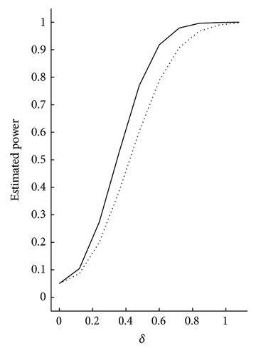
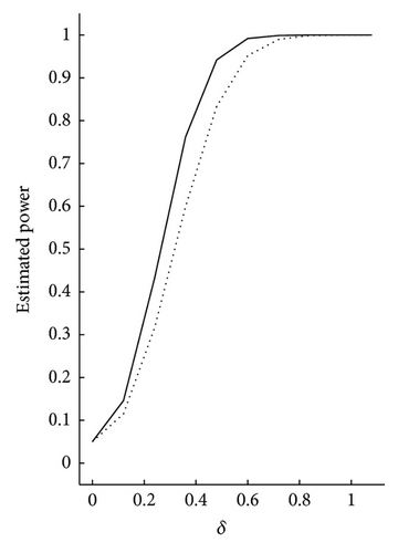
We first study the performance of the proposed testing procedure. Consider that the null hypothesis is H₀ : Aβ = 5 with A = (1,1) and the corresponding alternative hypothesis is H₁ : Aβ = 5 + δ with δ being a series of positive constants. For δ = 0, the alternative hypothesis becomes the null hypothesis. We take the bandwidths h₁ = h₂ = 0.8 · n^−1/5, the sample sizes n = 200,300, and . To illustrate the effectiveness of the proposed test statistics, the estimated power function curves with the significance level α = 0.05 are plotted for and . For each case, we repeat 1000 times. The results are given in Figure 1.

Details are in the caption following the image — **Figure 1 (a)**
Open in figure viewer PowerPoint

The plot of the estimated power function for sample sizes n = 200 and n = 300, where the solid line denotes n = 300 and the dotted line denotes n = 200. (a) shows the estimated power function curves with . (b) shows the estimated power function curves with .

From Figure 1, we can see the following results.

(1)
Our proposed test statistic is sensitive to the corresponding alternative hypothesis. This can be seen from the fact that if we increase the constant δ a little, the estimated power function increases rapidly.
(2)
The measurement errors affect the power function. For the same sample sizes, increasing the variance of the measurement error results in the decrease of the estimated power function. For the same measurement error, when the observation sample sizes increase, the estimated power function also increases. So our proposed procedure is feasible and easy to perform.

Second, we give the finite sample performance of the two-stage restricted estimator for nonparametric components with the restricted condition that Aβ = 5. For saving space, only the simulation results for estimators of f₁ are presented. We compare two estimators: one is the proposed two-stage restricted estimator for nonparametric component by (30) and the other is the benchmark estimator, which has the same form as the two-stage restricted estimator except that when we estimate f₁ we assume that f₂ is known. We use h₁ = h₂ = n^−1/5 to estimate

and the optimal bandwidth h chosen by the leave-one-out cross-validation method to estimate the nonparametric component f₁. The performance of estimators is evaluated by the root averaged squared errors (RASEs):

()

We take n = 200,300, 500 and

, respectively. For a given sample size, the sample means (SMs) and standard deviations (STDs) of RASEs are calculated. In each simulation, the repeated number is 1000. The simulation results are listed in Table 1.

Table 1. The finite sample performance of the estimators for f₁ under different sample sizes n and Σ_uu.

Σ_uu	n = 200	n = 300	n = 500
Σ_uu = 0.25I₂
Two-stage
SM	0.2249	0.1887	0.1530
STD	0.1152	0.0915	0.0552
Benchmark
SM	0.2239	0.1762	0.1494
STD	0.0958	0.0764	0.0533
Σ_uu = 0.4I₂
Two-stage
SM	0.2787	0.2298	0.1923
STD	0.1245	0.1077	0.0930
Benchmark
SM	0.2784	0.2284	0.1905
STD	0.1235	0.1043	0.0916
Σ_uu = 0.6I₂
Two-stage
SM	0.3253	0.2609	0.2162
STD	0.1728	0.1375	0.1038
Benchmark
SM	0.3200	0.2602	0.2153
STD	0.1707	0.1344	0.1008

From Table 1, it can be seen that, with the increase of the sample size n, the finite sample performance of the two estimators improves and the performance of the two-stage restricted estimator is close to that of the benchmark estimator. So the proposed two-stage restricted estimator of the nonparametric component has an oracle property.

5. Proofs

Firstly, some lemmas will be given.

Lemma 8. Let (X₁, Y₁), …, (X_n, Y_n) be i.i.d random vectors, where Y_i is scalar random variable. Further assume that E | Y|^s < ∞ and sup _x∫ | y|^sp(x, y)dy < ∞, where p(x, y) denotes the joint density of (X, Y). Let K(·) be a bounded positive function with a bounded support, satisfying a Lipschitz condition. Given that n^2δ−1h → ∞ for some δ < 1 − s⁻¹, then

()

This is Lemma 7.1 of Fan and Huang [17].

Lemma 9. Suppose that assumptions (A1)–(A5) hold. Then the following asymptotic approximations hold uniformly over all the elements of the matrices:

()

where d = 1,2. Similarly, the second formula is true for

This lemma is Lemma 3.1 and Lemma 3.2 of Opsomer and Ruppert [1].

Lemma 10. Suppose that assumptions (A1)–(A5) hold. Then as n → ∞, it holds that

()

where

The proof of this lemma can be found in the works of Wang et al. [10].

Lemma 11. Suppose that assumptions (A1)–(A5) hold. Then the corrected-profile least-squares estimatorof β is asymptotically normal. Namely,

()

This lemma is just Theorem 1 of Liang et al. [11] and is same as Theorem 3.2 of Wang et al. [10].

Proof of Theorem 1. Let

()

By Lemma 10, we can obtain

()

By the first equation of (18), we have

()

Using the results that J_n − J = o_P(1) and , we get

()

By the Slutsky theorem and Lemma 11, we can derive the result after some calculations.

Proof of Theorem 4. (1) Using Lemma 10, we know that

()

Similarly, we can prove that

()

Under the null hypothesis of testing problem (25) and by applying Lemma 11, we can prove that

()

By the second equation of (18), we get

()

Using (43), (31), and the Slutsky theorem, we derive that

()

By (43)–(45), it is easy to derive that, under the null hypothesis of testing problem (25),

()

(2) Under the alternative hypothesis and again by applying Lemma 11, we have

()

Using the similar argument as in (47), we can prove that

()

Then under the alternative hypothesis,we have

()

where χ²(k, ζ) denotes the asymptotic noncentral chi-squared distribution with k degrees of freedom and the noncentral parameter is

()

Proof of Theorem 6. Using (31), by some simple calculations, we get

()

where

()

Referring to the proof of Theorem 4.1 in Opsomer and Ruppert [1] and using Lemma 9, we obtain that

()

For Z_i1 in a small neighborhood of z₁ and |Z_i1 − z₁ | < h, for each f₁(Z_i1), we use the following Taylor expansion:

()

Then we derive that

()

By Lemma 8 and the usual nonparametric regression results, we can easily get

()

Using the result that

()

with H = diag (1, h), after some simple calculations, we can get

()

Note that

is asymptotically normal with mean 0 and variance

()

By the Slutsky theorem, we can derive that

()

Using similar calculation to that of T₂ and the result derived from Theorem 1 that , then we have

()

By using the Slutsky theorem again, we derive the desired result.

Acknowledgments

Wang’s researches are supported by the NSF project (ZR2011AQ007) of Shangdong Province of China and NNSF projects (11201499 and 11301309) of China.

References

1 Opsomer S. J. D. and Ruppert D., Fitting a bivariate additive model by local polynomial regression, Annals of Statistics. (1997) 25, no. 1, 186–211.
10.1214/aos/1034276626
Web of Science® Google Scholar
2 Li Q., Efficient estimation of additive partially linear models, International Economic Review. (2002) 41, no. 4, 1073–1092, https://doi.org/10.1111/1468-2354.00096, MR1790072.
10.1111/1468-2354.00096
Web of Science® Google Scholar
3 Jiang J., Zhou H., Jiang X., and Peng J., Generalized likelihood ratio tests for the structure of semiparametric additive models, The Canadian Journal of Statistics. (2007) 35, no. 3, 381–398, https://doi.org/10.1002/cjs.5550350304, MR2396026, ZBL1132.62025.
10.1002/cjs.5550350304
Web of Science® Google Scholar
4 Fuller W. A., Measurement Error Models, 1987, John Wiley & Sons, New York, NY, USA, https://doi.org/10.1002/9780470316665, MR898653.
10.1002/9780470316665
Google Scholar
5 Cheng C. L. and Van Ness J. W., Statistical Regression with Measurement Error, 1999, Arnold, London, UK, MR1719513, ZBL1235.76171.
Google Scholar
6 Carroll R. J., Ruppert D., Stefanski L. A., and Crainiceanu C. M., Measurement Error in Nonlinear Models, 2006, 2nd edition, Chapman and Hall, New York, NY, USA, https://doi.org/10.1201/9781420010138, MR2243417, ZBL1268.62129.
10.1201/9781420010138
Google Scholar
7 Liang H., Härdle W., and Carroll R. J., Estimation in a semiparametric partially linear errors-in-variables model, The Annals of Statistics. (1999) 27, no. 5, 1519–1535, https://doi.org/10.1214/aos/1017939140, MR1742498, ZBL0977.62036.
10.1214/aos/1017939140
Web of Science® Google Scholar
8 You J. and Chen G., Estimation of a semiparametric varying-coefficient partially linear errors-in-variables model, Journal of Multivariate Analysis. (2006) 97, no. 2, 324–341, https://doi.org/10.1016/j.jmva.2005.03.002, MR2234026, ZBL1085.62043.
10.1016/j.jmva.2005.03.002
Web of Science® Google Scholar
9 Li L. and Greene T., Varying coefficients model with measurement error, Biometrics. (2008) 64, no. 2, 519–526, https://doi.org/10.1111/j.1541-0420.2007.00921.x, MR2432422, ZBL1137.62397.
10.1111/j.1541-0420.2007.00921.x
CAS PubMed Web of Science® Google Scholar
10 Wang X., Chen F., and Lin L., Empirical likelihood inference for the parameter in additive partially linear EV models, Communications in Statistics. (2010) 39, no. 19, 3513–3524, https://doi.org/10.1080/03610920903315765, MR2747604, ZBL1202.62045.
10.1080/03610920903315765
Google Scholar
11 Liang H., Thurston S. W., Ruppert D., Apanasovich T., and Hauser R., Additive partial linear models with measurement errors, Biometrika. (2008) 95, no. 3, 667–678, https://doi.org/10.1093/biomet/asn024, MR2443182.
10.1093/biomet/asn024
Web of Science® Google Scholar
12 Jorgenson D. W., Econometric Modeling of Producer Behavior, 2000, MIT Press, Cambridge, Mass, USA, MR1821860.
10.7551/mitpress/2577.001.0001
Google Scholar
13 Wei C. and Wang Q., Statistical inference on restricted partially linear additive errors-in-variables models, Test. (2012) 21, no. 4, 757–774, https://doi.org/10.1007/s11749-011-0279-6, MR2992091.
10.1007/s11749-011-0279-6
Web of Science® Google Scholar
14 Wei C. H. and Wu X. Z., Profile Lagrange multiplier test for partially linear varying-coefficient regression models, Journal of Systems Science and Mathematical Sciences. (2008) 28, no. 4, 416–424, MR2425955.
Google Scholar
15 Zhang W., Li G., and Xue L., Profile inference on partially linear varying-coefficient errors-in-variables models under restricted condition, Computational Statistics & Data Analysis. (2011) 55, no. 11, 3027–3040, https://doi.org/10.1016/j.csda.2011.05.012, MR2813063, ZBL1218.62038.
10.1016/j.csda.2011.05.012
Web of Science® Google Scholar
16 Wei C. H. and Liu C., Statistical inference on semi-parametric partial linear additive models, Journal of Nonparametric Statistics. (2012) 24, no. 4, 809–823, https://doi.org/10.1080/10485252.2012.716155, MR2995478.
10.1080/10485252.2012.716155
Web of Science® Google Scholar
17 Fan J. and Huang T., Profile likelihood inferences on semiparametric varying-coefficient partially linear models, Bernoulli. (2005) 11, no. 6, 1031–1057, https://doi.org/10.3150/bj/1137421639, MR2189080, ZBL1098.62077.
10.3150/bj/1137421639
Web of Science® Google Scholar

All articles

Profile Inferences on Restricted Additive Partially Linear EV Models

Abstract

1. Introduction

2. Asymptotic Results of the Restricted-Profile Least-Squares Estimator and Modified Profile Lagrange Multiplier Test

2.1. The Restricted-Profile Least-Squares Estimator and Its Asymptotic Property

2.2. Modified Profile Lagrange Multiplier Test and Its Asymptotic Properties

3. Two-Stage Restricted Estimator for the Nonparametric Component

4. Simulation

5. Proofs

Acknowledgments

References

Figures

References

Information

About Wiley Online Library

Help & Support

Opportunities

Connect with Wiley

Profile Inferences on Restricted Additive Partially Linear EV Models

Abstract

1. Introduction

2. Asymptotic Results of the Restricted-Profile Least-Squares Estimator and Modified Profile Lagrange Multiplier Test

2.1. The Restricted-Profile Least-Squares Estimator and Its Asymptotic Property

2.2. Modified Profile Lagrange Multiplier Test and Its Asymptotic Properties

3. Two-Stage Restricted Estimator for the Nonparametric Component

4. Simulation

5. Proofs

Acknowledgments

References

Figures

References

Related

Information