A Posteriori Regularization Parameter Choice Rule for Truncation Method for Identifying the Unknown Source of the Poisson Equation
Abstract
We consider the problem of determining an unknown source which depends only on one variable in two-dimensional Poisson equation. We prove a conditional stability for this problem. Moreover, we propose a truncation regularization method combined with an a posteriori regularization parameter choice rule to deal with this problem and give the corresponding convergence estimate. Numerical results are presented to illustrate the accuracy and efficiency of this method.
1. Introduction
For the heat equation, there has been a large number of research results for the different forms of heat source [1–6]. In [7], the authors identified the unknown source of the Poisson equation using the modified regularization method. In [8], the authors identified the unknown source of the Poisson equation using the truncation method. In [7, 8], the regularization parameters which depend on the noise level and the a priori bound are selected by the a priori rule. Generally speaking, there is a defect for any a priori method; that is, the a priori choice of the regularization parameter depends seriously on the a priori bound E of the unknown solution. However, in general, the a priori bound E cannot be known exactly in practice, and working with a wrong constant E may lead to the bad regularized solution.
In the present paper, a posteriori choice of the regularization parameter will be given. To the authors’ knowledge, there are few papers for choosing the regularization parameter by the a posteriori rule for this problem.
The truncation regularization methods have been studied for solving various types of inverse problems. Eldén et al. [9] used the truncation method to analyze and compute one-dimensional IHCP, Xiong et al. [10] used it to consider the surface heat flux for the sideways heat equation, Fu et al. [11] used it to solve the BHCP, Qian et al. [12] used it to consider the numerical differentiation, and Regińska and Regiński [13] applied the idea of truncation to a Cauchy problem for the Helmholtz equation. In [9–13], the ill-posedness of the problem was caused by the high frequency components, and they all used the truncation method to eliminate all high frequencie and called this truncation method Fourier method. In [14], the authors ever identified the unknown source on Poisson equation on half unbounded domain using Fourier Transform. In this paper, we identified the unknown source on Poisson equation on half band domain using separation of variables and gave the numerical example to illustrate our methods. In [15], the authors ever used this method to consider a Cauchy problem for the Laplace equation in the bounded domain and obtained the error estimate which had a good convergence rate. The truncation method of this paper seems to be more direct and simple for considering the inverse problem in the bounded or half band domain.
This paper is organized as follows. The ill-posedness of this problem (1) is analyzed in Section 2. In Section 3, we give a conditional stable result. In Section 4, we propose the truncation method and give the convergence estimates under an a priori assumption for the exact solution and the a posteriori regularization parameter choice rule. In Section 5, a numerical example is proposed to show the effectiveness for this method. Section 6 puts an end to this paper with a brief conclusion.
2. Ill-Posedness of Problem (1)
3. A Conditional Stability Estimate
We firstly establish a conditional stability estimate for the inverse source problem (1).
Lemma 1. If n ≥ 1, one has the following inequality:
Theorem 2. Assume that f(x) is the solution of (1) and condition (11) is satisfied; then, the following estimate holds:
Remark 3. If f1, f2 are the solutions of the inverse source problem with exact data g1, g2, respectively, then there holds
4. An A Posteriori Regularization Parameter Choice Rule for the Truncation Method and Convergence Estimate
Lemma 4. Let condition (2) hold. If N is taken as the solution of (20), then one has the following inequality:
Proof. Due to (2) and (19), we obtain
The main conclusion of this paper is as the following.
Theorem 5. Let fδ,N(x) be the regularized solution given by (18), and let f(x) be the exact solution given by (10). Let gδ(x) be the measured data at y = 1 satisfying (2), and priori condition (11) holds for p > 0. If the regularization parameter N is chosen as the solution of (20), then one gets the following estimate:
Proof. Due to the triangle inequality, we obtain
5. Numerical Implementation
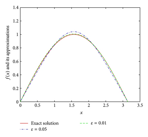
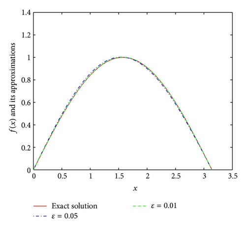
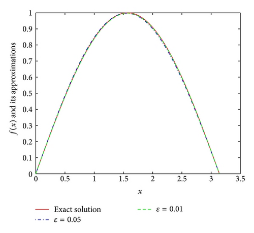
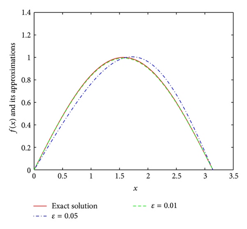
Example 6. It is easy to see that the function u(x, y) = (1 − e−y)sin x and the function f(x) = sinx are the exact solution of the problem (1). Consequently, the data function is g(x) = (1 − e−1)sin x.
Adding a random distributed perturbation to each data function, we obtain vector gδ; that is,
Using gδ as data function, we obtain the computed approximation fδ,N(x) by (19). The relative error er(f) is given by
From Figures 1, 2, 3, and 4, we find that the numerical results are quite satisfactory. Even with the noise level up to ε = 0.05, the numerical solutions are still in good agreement with the exact solution. In addition, the numerical results are better with the increase of p at first, but the numerical results are not so good after p = 3. This means that the numerical results are not so good for stronger “smoothness” assumptions on the exact solution f(x) which is consistent with the Tikhonov regularization method in [16]. These results are consistent with [8]. Comparing with [8], we can also easily find that the a posteriori parameter choice rule works better than the a priori parameter choice rule.
6. Conclusions
In this paper, a truncation regularization method is used to identify the unknown source term depending only on the spatial variable for the Poisson equation. The a posteriori rule for choosing regularization parameter with strict theory analysis is presented. In practice, the a priori bound is unknown exactly, and the regularization parameters can not be obtained exactly. This is a defect of the a priori rule for choosing regularization parameter. Using Morozov’s discrepancy principle, we give a posteriori parameter choice rule which depends only on the measured data. For the a posteriori parameter choice rule, we obtain the Hölder type error estimate.
Acknowledgment
The project is supported by the Distinguished Young Scholars Fund of Lanzhou University of Technology (Q201015).


