A Novel Method for Solving KdV Equation Based on Reproducing Kernel Hilbert Space Method
Abstract
We propose a reproducing kernel method for solving the KdV equation with initial condition based on the reproducing kernel theory. The exact solution is represented in the form of series in the reproducing kernel Hilbert space. Some numerical examples have also been studied to demonstrate the accuracy of the present method. Results of numerical examples show that the presented method is effective.
1. Introduction
The numerical solution of KdV equation is of great importance because it is used in the study of nonlinear dispersive waves. This equation is used to describe many important physical phenomena. Some of these studies are the shallow water waves and the ion acoustic plasma waves [4]. It represents the long time evolution of wave phenomena, in which the effect of nonlinear terms uux is counterbalanced by the dispersion uxxx. Thus it has been found to model many wave phenomena such as waves in enharmonic crystals, bubble liquid mixtures, ion acoustic wave, and magnetohydrodynamic waves in a warm plasma as well as shallow water waves [5, 6].
The KdV equation exhibits solutions such as solitary waves, solitons and recurrence [7]. Goda [8] and Vliengenthart [9] used the finite difference method to obtain the numerical solution of KdV equation. Soliman [2] used the collocation solution with septic splines to obtain the solution of the KdV equation. Numerical solutions of KdV equation were obtained by the variational iteration method, finite difference method [3, 10], and by using the meshless based on the collocation with radial basis functions [11]. Wazwaz presented the Adomian decomposition method for KdV equation with different initial conditions [12]. Syam [13] worked the ADM for solving the nonlinear KdV equation with appropriate initial conditions.
The theory of reproducing kernels was used for the first time at the beginning of the 20th century by Zaremba in his work on boundary value problems for harmonic and biharmonic functions [14]. Reproducing kernel theory has important application in numerical analysis, differential equations, probability and statistics [14, 15]. Recently, using the RKM, some authors discussed fractional differential equation, nonlinear oscillator with discontinuity, singular nonlinear two-point periodic boundary value problems, integral equations, and nonlinear partial differential equations [14, 15].
The efficiency of the method was used by many authors to investigate several scientific applications. Geng and Cui [16] applied the RKHSM to handle the second-order boundary value problems. Yao and Cui [17] and Wang et al. [18] investigated a class of singular boundary value problems by this method and the obtained results were good. Zhou et al. [19] used the RKHSM effectively to solve second-order boundary value problems. In [20], the method was used to solve nonlinear infinite-delay-differential equations. Wang and Chao [21], Li and Cui [22], and Zhou and Cui [23] independently employed the RKHSM to variable-coefficient partial differential equations. Geng and Cui [24] and Du and Cui [25] investigated to the approximate solution of the forced Duffing equation with integral boundary conditions by combining the homotopy perturbation method and the RKHSM. Lv and Cui [26] presented a new algorithm to solve linear fifth-order boundary value problems. In [27, 28], authors developed a new existence proof of solutions for nonlinear boundary value problems. Cui and Du [29] obtained the representation of the exact solution for the nonlinear Volterra-Fredholm integral equations by using the reproducing kernel space. Wu and Li [30] applied iterative reproducing kernel method to obtain the analytical approximate solution of a nonlinear oscillator with discontinuities. Inc et al. [15] used this method for solving Telegraph equation.
The paper is organized as follows. Section 2 introduces several reproducing kernel spaces and a linear operator. The representation in W(Ω) is presented in Section 3. Section 4 provides the main results. The exact and approximate solutions of (1) and (2) and an iterative method are developed for the kind of problems in the reproducing kernel space. We have proved that the approximate solution uniformly converges to the exact solution. Some numerical experiments are illustrated in Section 5. We give some conclusions in Section 6.
2. Preliminaries
2.1. Reproducing Kernel Spaces
In this section, we define some useful reproducing kernel spaces.
Definition 1 (reproducing kernel). Let E be a nonempty abstract set. A function K : E × E → C is a reproducing kernel of the Hilbert space H if and only if
- (a)
for all t ∈ E, K(·, t) ∈ H,
- (b)
for all t ∈ E, φ ∈ H, 〈φ(·), K(·, t)〉 = φ(t). This is also called “the reproducing property”: the value of the function φ at the point t is reproduced by the inner product of φ with K(·, t).
Theorem 2. The space is a complete reproducing kernel space and, its reproducing kernel function Ry(x) can be denoted by
Proof. Since
Theorem 3. The W(Ω) is a reproducing kernel space, and its reproducing kernel function is
3. Solution Representation in W(Ω)
Lemma 4. The operator L is a bounded linear operator.
Proof. We have
Theorem 5. Suppose that is dense in Ω; then is complete system in W(Ω) and
Proof. We have
Theorem 6. If is dense in Ω, then the solution of (39) is
Proof. Since is complete system in W(Ω), we have
4. The Method Implementation
Lemma 7. If , (xn, tn)→(y, s), and f(x, t, v(x, t), vx(x, t)) is continuous, then
Proof. Since
From the definition of the reproducing kernel, we have
Theorem 8. Suppose that ∥vn∥ is a bounded in (58) and (39) has a unique solution. If is dense in Ω, then the n-term approximate solution vn(x, t) derived from the above method converges to the analytical solution v(x, t) of (39) and
Proof. First, we prove the convergence of vn(x, t). From (58), we infer that
5. Numerical Results
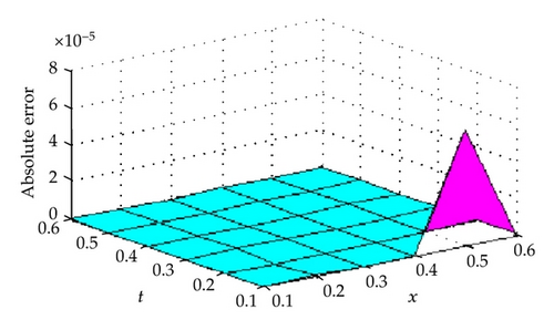
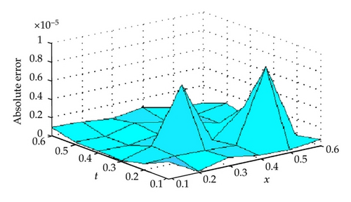
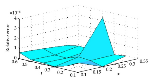
In this section, two numerical examples are provided to show the accuracy of the present method. All computations are performed by Maple 16. Results obtained by the method are compared with exact solution and the ADM [13] of each example are found to be in good agreement with each others. The RKM does not require discretization of the variables, that is, time and space, it is not effected by computation round off errors and one is not faced with necessity of large computer memory and time. The accuracy of the RKM for the KdV equation is controllable and absolute errors are very small with present choice of x and t (see Tables 1, 2, 3, and 4 and Figures 1, 2, and 3). The numerical results that we obtained justify the advantage of this methodology.
| x/t | 0.1 | 0.2 | 0.3 | 0.4 | 0.5 | 0.6 |
|---|---|---|---|---|---|---|
| 0.1 | 1.830273924 | 1.269479180 | 0.718402632 | 0.36141327 | 0.17121984 | 0.07882210 |
| 0.2 | 1.922085966 | 1.423155525 | 0.839948683 | 0.43230491 | 0.20711674 | 0.09585068 |
| 0.3 | 1.980132581 | 1.572895466 | 0.973834722 | 0.51486639 | 0.25001974 | 0.11644607 |
| 0.4 | 2 | 1.711277572 | 1.118110335 | 0.61003999 | 0.30105415 | 0.14130164 |
| 0.5 | 1.980132581 | 1.830273924 | 1.269479180 | 0.71840263 | 0.36141327 | 0.17121984 |
| 0.6 | 1.922085966 | 1.922085966 | 1.423155525 | 0.83994868 | 0.43230491 | 0.20711674 |
| x/t | 0.1 | 0.2 | 0.3 | 0.4 | 0.5 | 0.6 |
|---|---|---|---|---|---|---|
| 0.1 | 1.830273864 | 1.269478141 | 0.718402628 | 0.36141327 | 0.17128272 | 0.07883011 |
| 0.2 | 1.922085928 | 1.423155537 | 0.839948629 | 0.43230491 | 0.20711710 | 0.09585155 |
| 0.3 | 1.980132606 | 1.572896076 | 0.973834717 | 0.51486633 | 0.25001974 | 0.11644677 |
| 0.4 | 2.000000027 | 1.711278098 | 1.118110380 | 0.61004008 | 0.30105468 | 0.14130128 |
| 0.5 | 1.980133013 | 1.830274266 | 1.269479288 | 0.71840299 | 0.36141338 | 0.17122050 |
| 0.6 | 1.922086667 | 1.922086057 | 1.423155510 | 0.83994874 | 0.43230465 | 0.20711669 |
| x/t | 0.1 | 0.2 | 0.3 | 0.4 | 0.5 | 0.6 |
|---|---|---|---|---|---|---|
| 0.1 | 1.78 × 10⁻⁶ | 3.01 × 10⁻⁹ | 8.55 × 10⁻⁷ | 3.49 × 10⁻⁷ | 2.85 × 10⁻⁷ | 6.28 × 10⁻⁷ |
| 0.2 | 6.38 × 10⁻⁷ | 6.98 × 10⁻⁷ | 6.52 × 10⁻⁷ | 4.51 × 10⁻⁷ | 8.33 × 10⁻⁶ | 2.42 × 10⁻⁷ |
| 0.3 | 2.2 × 10⁻⁸ | 9.09 × 10⁻⁷ | 6.88 × 10⁻⁶ | 1.35 × 10⁻⁷ | 2.97 × 10⁻⁶ | 1.69 × 10⁻⁷ |
| 0.4 | 1.70 × 10⁻⁷ | 1.03 × 10⁻⁷ | 5.38 × 10⁻⁷ | 1.20 × 10⁻⁶ | 3.98 × 10⁻⁷ | 1.68 × 10⁻⁷ |
| 0.5 | 2.26 × 10⁻⁷ | 1.29 × 10⁻⁷ | 8.74 × 10⁻⁷ | 3.13 × 10⁻⁷ | 4.02 × 10⁻⁷ | 9.63 × 10⁻⁷ |
| 0.6 | 8.94 × 10⁻⁷ | 7.83 × 10⁻⁷ | 4.34 × 10⁻⁷ | 9.79 × 10⁻⁷ | 2.77 × 10⁻⁷ | 1.45 × 10⁻⁸ |
| x/t | 0.1 | 0.2 | 0.3 | 0.4 | 0.5 | 0.6 |
|---|---|---|---|---|---|---|
| 0.1 | 9.201 × 10⁻⁷ | 5.113 × 10⁻¹⁰ | 5.707 × 10⁻⁷ | 3.868 × 10⁻⁷ | 6.06 × 10⁻⁷ | 2.76 × 10⁻⁶ |
| 0.2 | 3.441 × 10⁻⁷ | 3.498 × 10⁻⁷ | 3.968 × 10⁻⁷ | 4.320 × 10⁻⁷ | 1.48 × 10⁻⁶ | 8.84 × 10⁻⁷ |
| 0.3 | 1.255 × 10⁻⁸ | 4.555 × 10⁻⁷ | 3.881 × 10⁻⁶ | 1.132 × 10⁻⁷ | 4.49 × 10⁻⁶ | 5.13 × 10⁻⁷ |
| 0.4 | 1.032 × 10⁻⁷ | 5.264 × 10⁻⁸ | 2.862 × 10⁻⁷ | 8.964 × 10⁻⁷ | 5.13 × 10⁻⁷ | 4.27 × 10⁻⁷ |
| 0.5 | 1.460 × 10⁻⁷ | 6.857 × 10⁻⁸ | 4.469 × 10⁻⁷ | 2.089 × 10⁻⁷ | 4.44 × 10⁻⁷ | 2.04 × 10⁻⁶ |
| 0.6 | 6.079 × 10⁻⁷ | 4.410 × 10⁻⁷ | 2.175 × 10⁻⁷ | 5.958 × 10⁻⁷ | 2.65 × 10⁻⁷ | 2.58 × 10⁻⁸ |


Example 10 (see [13].)Consider the following KdV equation with initial condition
Example 11 (see [13].)We now consider the KdV equation with initial condition
Remark 12. The problem discussed in this paper has been solved with Adomian method [13] and Homotopy analysis method [31]. In these studies, even though the numerical results give good results for large values of x, these methods give away values from the analytical solution for small values of x and t. However, the method is used in our study for large and small values of x and t, results are very close to the analytical solutions can be obtained. In doing so, it is possible to refine the result by increasing the intensive points.
6. Conclusion
In this paper, we introduce an algorithm for solving the KdV equation with initial condition. For illustration purposes, we chose two examples which were selected to show the computational accuracy. It may be concluded that the RKM is very powerful and efficient in finding exact solution for wide classes of problem. The approximate solution obtained by the present method is uniformly convergent.
Clearly, the series solution methodology can be applied to much more complicated nonlinear differential equations and boundary value problems. However, if the problem becomes nonlinear, then the RKM does not require discretization or perturbation and it does not make closure approximation. Results of numerical examples show that the present method is an accurate and reliable analytical method for the KdV equation with initial or boundary conditions.
Acknowledgment
A. Kiliçman gratefully acknowledge that this paper was partially supported by the University Putra Malaysia under the ERGS Grant Scheme having project no. 5527068 and Ministry of Science, Technology and Inovation (MOSTI), Malaysia under the Science Fund 06-01-04-SF1050.


