Volume 2013, Issue 1 562140

Research Article

Open Access

Numerical Solution of the Fractional Partial Differential Equations by the Two-Dimensional Fractional-Order Legendre Functions

Fukang Yin,

Corresponding Author

Fukang Yin

[email protected]

orcid.org/0000-0002-8353-7000

College of Computer, National University of Defense Technology, Changsha 410073, China nudt.edu.cn

Search for more papers by this author

Junqiang Song,

Junqiang Song

College of Computer, National University of Defense Technology, Changsha 410073, China nudt.edu.cn

Search for more papers by this author

Yongwen Wu,

Yongwen Wu

College of Computer, National University of Defense Technology, Changsha 410073, China nudt.edu.cn

Search for more papers by this author

Lilun Zhang,

Lilun Zhang

College of Computer, National University of Defense Technology, Changsha 410073, China nudt.edu.cn

Search for more papers by this author

Fukang Yin,

Corresponding Author

Fukang Yin

[email protected]

orcid.org/0000-0002-8353-7000

College of Computer, National University of Defense Technology, Changsha 410073, China nudt.edu.cn

Search for more papers by this author

Junqiang Song,

Junqiang Song

College of Computer, National University of Defense Technology, Changsha 410073, China nudt.edu.cn

Search for more papers by this author

Yongwen Wu,

Yongwen Wu

College of Computer, National University of Defense Technology, Changsha 410073, China nudt.edu.cn

Search for more papers by this author

Lilun Zhang,

Lilun Zhang

College of Computer, National University of Defense Technology, Changsha 410073, China nudt.edu.cn

Search for more papers by this author

First published: 18 November 2013

https://doi.org/10.1155/2013/562140

Citations: 18

Academic Editor: Santanu Saha Ray

Share a link

Email
Wechat
Bluesky

Abstract

A numerical method is presented to obtain the approximate solutions of the fractional partial differential equations (FPDEs). The basic idea of this method is to achieve the approximate solutions in a generalized expansion form of two-dimensional fractional-order Legendre functions (2D-FLFs). The operational matrices of integration and derivative for 2D-FLFs are first derived. Then, by these matrices, a system of algebraic equations is obtained from FPDEs. Hence, by solving this system, the unknown 2D-FLFs coefficients can be computed. Three examples are discussed to demonstrate the validity and applicability of the proposed method.

1. Introduction

Fractional partial differential equations play a significant role in modeling physical and engineering processes. Therefore, there is an urgent need to develop efficient and fast convergent methods for FPDEs. Recently, several different techniques, including Adomian’s decomposition method (ADM) [1, 2], homotopy perturbation method (HPM) [3–5], variational iteration method (VIM) [6–8], spectral methods [9–13], orthogonal polynomials method [14–17], and wavelets method [18–21] have been presented and applied to solve FPDEs.

The method based on the orthogonal functions is a wonderful and powerful tool for solving the FDEs and has enjoyed many successes in this realm. The operational matrix of fractional integration has been determined for some types of orthogonal polynomials, such as Chebyshev polynomials [16], Legendre polynomials [22], Laguerre polynomials [23–25], and Jacobi polynomials [26]. Moreover, the operational matrix of fractional derivative for Chebyshev polynomials [9] and Legendre polynomials [9, 14] also has been derived. However, since these polynomials using integer power series to approximate fractional ones, it cannot accurately represent properties of fractional calculus. Recently, Rida and Yousef [27] presented a fractional extension of the classical Legendre polynomials by replacing the integer order derivative in Rodrigues formula with fractional order derivatives. The defect is that the complexity of these functions made them unsuitable for solving FDEs. Subsequently, Kazem et al. [28] presented the orthogonal fractional order Legendre functions based on shifted Legendre polynomials to find the numerical solution of FDEs and drew a conclusion that their method is accurate, effective, and easy to implement.

Benefiting from their “exponential-convergence” property when smooth solutions are involved, spectral methods have been widely and effectively used for the numerical solution of partial differential equations. The basic idea of spectral methods is to expand a function into sets of smooth global functions, called the trial functions. Because of their special properties, the orthogonal polynomials are usually chosen to be trial functions. Spectral methods can obtain very accurate approximations for a smooth solution while only need a few degrees of freedom. Recently, Chebyshev spectral method [9], Legendre spectral method [10], and adaptive pseudospectral method [11] were proposed for solving fractional boundary value problems. Moreover, generalized Laguerre spectral algorithms and Legendre spectral Galerkin method were developed by Baleanu et al. [12] and Bhrawy and Alghamdi [13] for fractional initial value problems, respectively.

Motivated and inspired by the ongoing research in orthogonal polynomials methods and spectral methods, we construct two-dimensional fractional-order Legendre functions and derive the operational matrices of integration and derivative for the solution of FPDEs. To the best of the authors’ knowledge, such approach has not been employed for solving FPDEs.

The rest of the paper is organized as follows. In Section 2, we introduce some mathematical preliminaries of the fractional calculus theory and fractional-order Legendre functions. In Section 3, a basis of 2D-FLFs is defined and some properties are given. Section 4 is devoted to the operational matrices of fractional derivative and integration for 2D-FLFs. Some numerical examples are presented in Section 5. Finally, we conclude the paper with some remarks.

2. Preliminaries and Notations

2.1. Fractional Calculus Theory

Some necessary definitions and Lemma of the fractional calculus theory [29, 30] are listed here for our subsequent development.

Definition 1. A real function h(t), t > 0, is said to be in the space C_μ, μ ∈ R, if there exists a real number p > μ, such that h(t) = t^ph₁(t), where h₁(t) ∈ C(0, ∞), and it is said to be in the space if and only if h⁽ⁿ⁾ ∈ C_μ, n ∈ N.

Definition 2. Riemann-Liouville fractional integral operator (J^α) of order α ≥ 0, of a function f ∈ C_μ, μ ≥ −1 is defined as

()

where Γ(α) is the well-known Gamma function. Some properties of the operator J^α can be found, for example, in [29, 30].

Definition 3. The fractional derivative of f(x) in the Caputo sense is defined as

()

where f : R → R, x → f(x) denotes a continuous (but not necessarily differentiable) function.

Lemma 4. Let n − 1 < α ≤ n, n ∈ N, t > 0, , μ ≥ −1. Then

()

2.2. Fractional-Order Legendre Functions

In this section, we introduce the fractional-order Legendre functions which were first proposed by Kazem et al. [28]. The normalized eigenfunctions problem for FLFs is

()

which is a singular Sturm-Liouville problem. The fractional-order Legendre polynomials, denoted by

, are defined on the interval [0,1] and can be determined with the aid of following recurrence formulae:

()

and the analytic form of

of degree i is given by

()

where

and

. The orthogonality condition is

()

where ω(x) = x^α−1 is the weight function and δ is the Kronecker delta. For more details, please see [28].

3. 2D-FLFs

In this section, the definitions and theorems of 2D-FLFs are given by Liu’s method described in [31].

3.1. Definitions and Properties of the 2D-FLFs

Definition 5. Let be the fractional Legendre polynomials on [0,1]; we call the two-dimensional fractional Legendre polynomials on [0,1] × [0,1].

Theorem 6. The basis is orthogonal on [0,1] × [0,1] with the weight function ω(x, y) = ω(x)ω(y) = x^α−1y^β−1.

Proof. Let i ≠ m or j ≠ n

()

Theorem 7. Consider

()

3.2. 2D-FLFs Expansion

Definition 8. A function of two independent variables f(x, y) which is integrable in square [0,1] × [0,1] can be expanded as

()

where

()

Theorem 9. If the series converges uniformly to f(x, y) on the square [0,1] × [0,1], then we have

()

Proof. By multiplying on both sides of (10), where n and m are fixed and integrating termwise with regard to x and y on [0,1] × [0,1], then

()

Finally one can get (11).

If the infinite series in (10) is truncated, then it can be written as

()

where C and Ψ(x^α, y^β) are given by

()

where

, i = 0,1, …, m, and j = 0,1, …, m^′.

According to the definition of FLFs, one can find that fractional Legendre polynomials are identical to Legendre polynomials shifted to [0,1] when using the transform x^α → x, y^β → y. Therefore, in a similar method described in [31], we can easily get the convergence and stability theorems of proposed method.

Lemma 10. If the function f(x, y) is a continuous function on [0,1] × [0,1] and the series converges uniformly to f(x, y), then is the 2D-FLFs expansion of f(x, y).

Proof (by contradiction). Let

()

Then there is at least one coefficient such that a_nm ≠ b_nm. However,

()

Lemma 11. If two continuous functions defined on [0,1] × [0,1] have the identical 2D-FLFs expansions, then these two functions are identical.

Proof. Suppose that f(x, y) and g(x, y) can be expanded by 2D-FLFs as follows:

()

By subtracting the above two equations with each other, one has

()

Then Lemma 11 can be proved.

Theorem 12. If the 2D-FLFs expansion of a continuous function f(x, y) converges uniformly, then the 2D-FLFs expansion converges to the function f(x, y).

Proof. Theorem 12 can be proved by Theorems 7 and 9.

Theorem 13. If the sum of the absolute values of the 2D-FLFs coefficients of a continuous function f(x, y) forms a convergent series, then the 2D-FLFs expansion is absolutely uniformly convergent, and converges to the function f(x, y).

Proof. Consider

()

Then

converges uniformly to the function f(x, y).

Theorem 14. If a continuous function f(x, y), defined on [0,1] × [0,1], has bounded mixed partial derivative , then the 2D-FLFs expansion of the function converges uniformly to the function.

Proof. Let f(x, y) be a function defined on [0,1] × [0,1] such that

()

where M is a positive constant and

()

By employing the transform X = 2x^α − 1 and Y = 2y^β − 1, one can obtain

()

Consequently, in a similar method described in [31], Theorem 14 can be proved.

4. Operational Matrices of 2D-FLFs

4.1. Integration Operational Matrices of 2D-FLFs

Lemma 15. The Riemann-Liouville fractional integration of order γ > 0 of the 2D-FLFs ψ_ij can be obtained in the form of

()

Proof. Consider

()

Lemma 16. Let γ > 0; then one has

()

Proof. Using previous Lemma 15 and (6), one can have

()

Theorem 17. Let Ψ(x^α, y^β) be the 2D-FLFs vector defined in (16); then one has

()

where

is the mm^′ × mm^′ operational matrix of Riemann-Liouville fractional integration of order γ > 0, and has the form as follows:

()

in which

is m^′ × m^′ matrix and the elements are defined as follows:

()

and I is m^′ × m^′ identity matrix.

Proof. Using (29) and orthogonality property of FLFs, one can get

()

where

and H⁻¹ are two m^′ × m^′ matrices defined as

()

Now by substituting above equations in (32), Theorem 12 can be proved.

In a similar way as previous, one can obtain the operational matrix of Riemann-Liouville fractional integration with respect to variable y.

Theorem 18. Let Ψ(x^α, y^β) be the 2D-FLFs vector defined in (16); one has

()

where

is the mm^′ × mm^′ operational matrix of Riemann-Liouville fractional integration of order γ > 0, and has the form as follows:

()

in which E is m^′ × m^′ matrix and the elements are defined as follows:

()

4.2. Derivative Operational Matrices of 2D-FLFs

Lemma 19. The FLFs Caputo fractional derivative of γ > 0 can be obtained in the form of

()

where

when sα ∈ N₀ and sα < γ in other case

Proof. Consider

()

Lemma 20. Let γ > 0, α ∉ N; then one has

()

Proof. Using previous Lemma 19 and (6), one can have

()

Theorem 21. Let Ψ(x^α, y^β) be the 2D-FLFs vector defined in (16); one has

()

where

is the mm^′ × mm^′ operational matrix of Caputo fractional derivative of order γ > 0, and has the form as follows:

()

in which

is m^′ × m^′ matrix and the elements are defined as follows:

()

and I is a m^′ × m^′ identity matrix.

Proof. Using (41) and the orthogonality property of FLFs, one can have

()

where

and H⁻¹ are two mm^′ × mm^′ matrices defined as

()

Now by substituting above equations in (44), Theorem 21 can be proved.

In a similar way as above, one can get Caputo fractional derivative of order γ > 0 with respect to variable y.

Theorem 22. Let Ψ(x^α, y^β) be the 2D-FLFs vector defined in (16); one can have

()

where

is the mm^′ × mm^′ operational matrix of Caputo fractional derivative of order γ > 0, and has the form as follows:

()

in which F is m^′ × m^′ matrix and the elements are defined as follows:

()

5. Applications and Results

Consider the following FPDEs:

()

where L and N are linear operator and nonlinear operator; respectively. D^α and D^β are the Caputo fractional derivatives of order α and β, respectively; g is a known analytic function.

By employing operator

on both sides of (49) and then using the Lemma 4, one can have

()

We first express unknown function u(x, t) and derivative term

()

Now for the nonlinear part, by employing the nonlinear term approximation method described in [32] and then by using transform x → x^α, t → t^β, one can get the 2D-FLFs expansion of nonlinear term as

()

where N^T is coefficient matrix of nonlinear term which must be computed and its order is mm^′ × mm^′.

For the linear part, we have

()

where L is a matrix of order mm^′ × mm^′.

After substituting (51)–(53) into (50), one can obtain

()

According to the Wu’s [33] technology for determining the initial iteration value, the initial iteration value is chosen as

. The coefficient matrix C^T can be computed by using the MATLAB function fsolve( ) or the method described in [34].

Now, the present method is applied to solve the linear and nonlinear FPDEs, and their results are compared with the solution of other methods. The accuracy of our approach is estimated by the following error functions:

()

Example 23. Consider the one-dimensional linear inhomogeneous fractional Burger’s equation [35]:

()

with the initial condition u(x, 0) = x² and the exact solution being u(x, t) = x² + t².

By employing 2D-FLFs method, one can get

()

where α = 1. Then we can get

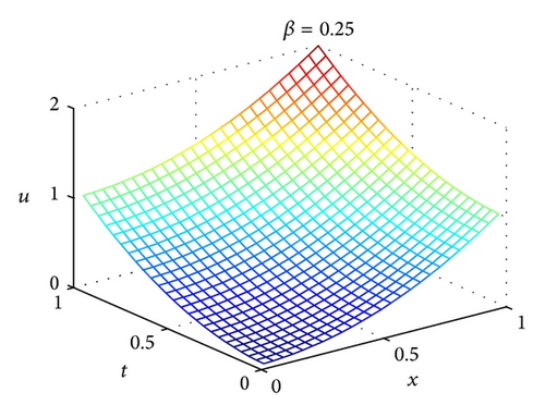
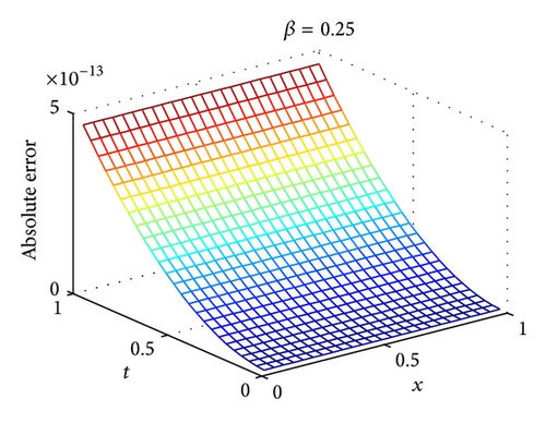
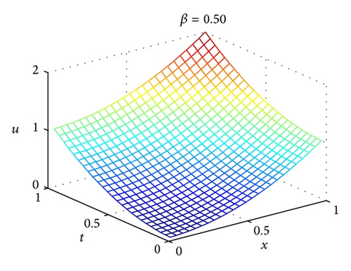
Figures 1(a) and 1(b) show the numerical results for β = 0.25 with m = 3, m^′ = 9 and β = 0.5 with m = 3, m^′ = 5, respectively. It should be found that the accuracy of 2D-FLFs method is very high while only a small number of 2D-FLFs are needed.

Details are in the caption following the image — **Figure 1 (a)**
Open in figure viewer PowerPoint

Numerical results for Example 23 when β = 0.25, 0.50.

Example 24. Consider nonlinear fractional Klein-Gordon equation [36, 37]:

()

subject to the initial conditions

()

and g(x, t) = Γ(β + 1)x^α − Γ(α + 1)t^β + x^3αt^3β. The exact solution of (58) is u(x, t) = x^αt^β.

By employing 2D-FLFs method with m = 3 and m^′ = 3, one can have

()

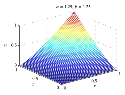
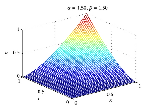
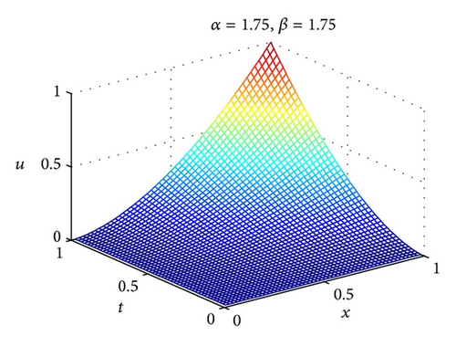
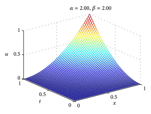
The numerical results of Example 24 for different values of α and β are shown in Figure 2. In addition, L₂ and L_∞ errors are presented in Table 1. From Table 1, one can conclude that the solutions of 2D-FLFs method are in good agreement with the exact results. Compared with homotopy analysis method (HAM) [36] and homotopy perturbation method (HPM) [37], 2D-FLFs method can get high accuracy solution while only need a few terms of 2D-FLFs.

Table 1. Errors of Example 24 for different values of α and β with M = M^′ = 4.

Error	α = β = 1.25	α = β = 1.50	α = β = 1.75	α = β = 2.00
L₂	5.6437e − 015	1.2075e − 015	3.4584e − 015	8.9917e − 016
L_∞	4.4409e − 016	1.1102e − 016	3.3307e − 016	1.1102e − 016

Example 25. Consider the nonlinear time-fractional advection partial differential equation [37–39]

()

subject to the initial condition

()

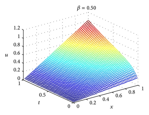
Figure 3 gives the approximation solutions of (61) for β = 0.50 with m = 4, m^′ = 5 and β = 0.75 with m = 4, m^′ = 9. Moreover, Table 2 shows the approximate solutions for (61) obtained for different values of β using the fractional variational iteration method (FVIM) [39] and 2D-FLFs method. The values of β = 1 are the only case for which we know the exact solution u(x, t) = xt. It should be noted that only the fourth-order term of the FVIM was used in evaluating the approximate solutions for Table 2. From Table 2, it clearly appears that 2D-FLFs method is more accurate than FVIM and the obtained results are in good agreement with exact solution.

Table 2. Numerical values when β = 0.50, 0.75, and 1.0 for (61).

t	x	β = 0.50		β = 0.75		β = 1.00
t	x	FVIM	2D-FLFs	FVIM	2D-FLFs	FVIM	2D-FLFs	Exact
0.25	0.25	0.12422501	0.12225461	0.09230374	0.09224583	0.06250058	0.062500	0.062500
	0.50	0.24845002	0.24450922	0.18460748	0.18449165	0.12500117	0.125000	0.125000
	0.75	0.37267504	0.36676383	0.27691122	0.27673748	0.18750175	0.187500	0.187500
	1.00	0.49690005	0.48901844	0.36921496	0.36898331	0.25000234	0.250000	0.250000

0.50	0.25	0.18377520	0.16584130	0.15148283	0.14985508	0.12507592	0.125000	0.125000
	0.50	0.36755040	0.33168259	0.30296566	0.29971016	0.25015184	0.250000	0.250000
	0.75	0.55132559	0.49752389	0.45444848	0.44956524	0.37522776	0.375000	0.375000
	1.00	0.73510079	0.66336518	0.60593131	0.59942032	0.50030368	0.500000	0.500000

0.75	0.25	0.27227270	0.20678964	0.21407798	0.20119503	0.18881843	0.187500	0.187500
	0.50	0.54454540	0.41357929	0.42815596	0.40239005	0.37763687	0.375000	0.375000
	0.75	0.81681810	0.62036893	0.64223394	0.60358508	0.56645530	0.562500	0.562500
	1.00	1.08909080	0.82715857	0.85631192	0.80478011	0.75527373	0.750000	0.750000

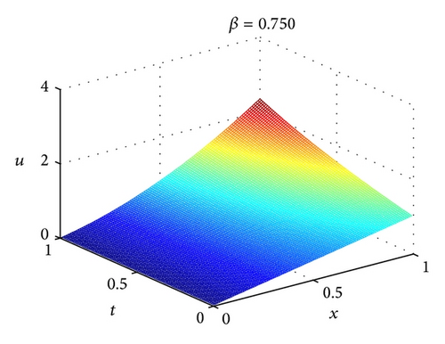
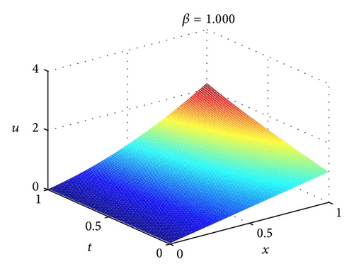
Example 26. We finally consider the linear time-fractional wave equation:

()

subject to the initial conditions

()

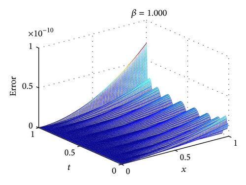
Table 3 gives a comparison of the approximate solutions at different values of β using the FVIM [39] and 2D-FLFs method. Figure 4 shows the numerical solutions of 2D-FLFs method for (63) at different values of β with m = 3, m^′ = 9. The values of β = 1 are the only case for which we know the exact solution u(x, t) = x + x²sinh (t). As previous, only the fourth-order term of the FVIM was used in evaluating the numerical solutions for Table 3. In the case of β = 1, it can be found that absolute error of 2D-FLFs is not bigger than 1.0e − 10 which is very small compared with that obtained by FVIM.

Table 3. Numerical values when β = 0.750, 0.875, and 1.000 for (63).

t	x	β = 0.750		β = 0.875		β = 1.000
t	x	FVIM	2D-FLFs	FVIM	2D-FLFs	FVIM	Exact
0.25	0.25	0.26622298	0.26622021	0.26593959	0.26594005	0.26578827	0.26578827
	0.50	0.56489190	0.56488083	0.56375836	0.56376020	0.56315308	0.56315308
	0.75	0.89600678	0.89598187	0.89345630	0.89346046	0.89209443	0.89209443
	1.00	1.25956762	1.25952332	1.25503343	1.25504082	1.25261232	1.25261232

0.50	0.25	0.28474208	0.28474415	0.28340402	0.28340659	0.28256846	0.28256846
	0.50	0.63896831	0.63897662	0.63361610	0.63362636	0.63027383	0.63027383
	0.75	1.06267869	1.06269739	1.05063622	1.05065931	1.04311611	1.04311611
	1.00	1.55587323	1.55590647	1.53446439	1.53450544	1.52109530	1.52109531

0.75	0.25	0.30690489	0.30690747	0.30361709	0.30361656	0.30139478	0.30139480
	0.50	0.72761955	0.72762986	0.71446834	0.71446625	0.70557913	0.70557918
	0.75	1.26214400	1.26216719	1.23255378	1.23254905	1.21255304	1.21255316
	1.00	1.91047821	1.91051944	1.85787338	1.85786498	1.82231652	1.82231673

6. Conclusion

We define a basis of 2D-FLFs and derived its operational matrices of fractional derivative and integration, which are used to approximate the numerical solution of FPDEs. Compared with other numerical methods, 2D-FLFs method can accurately represent properties of fractional calculus. Moreover, only a small number of 2D-FLFs are needed to obtain a satisfactory result. The obtained results demonstrate the validity and applicability of proposed method for solving the FPFEs.

Acknowledgments

This work is supported by the National Natural Science Foundation of China (Grant no. 11272352). The authors are grateful to the anonymous referees for their comments which substantially improved the quality of this paper.

References

1 Odibat Z. and Momani S., Numerical methods for nonlinear partial differential equations of fractional order, Applied Mathematical Modelling. (2008) 32, no. 1, 28–39, 2-s2.0-34548384362, https://doi.org/10.1016/j.apm.2006.10.025.
10.1016/j.apm.2006.10.025
Web of Science® Google Scholar
2 Momani S. and Odibat Z., Analytical approach to linear fractional partial differential equations arising in fluid mechanics, Physics Letters A. (2006) 355, no. 4-5, 271–279, 2-s2.0-33646878106, https://doi.org/10.1016/j.physleta.2006.02.048.
10.1016/j.physleta.2006.02.048
CAS Web of Science® Google Scholar
3 Odibat Z. and Momani S., Modified homotopy perturbation method: application to quadratic Riccati differential equation of fractional order, Chaos, Solitons & Fractals. (2008) 36, no. 1, 167–174, https://doi.org/10.1016/j.chaos.2006.06.041, MR2372056, ZBL1152.34311.
10.1016/j.chaos.2006.06.041
Web of Science® Google Scholar
4 Hosseinnia S. H., Ranjbar A., and Momani S., Using an enhanced homotopy perturbation method in fractional differential equations via deforming the linear part, Computers & Mathematics with Applications. (2008) 56, no. 12, 3138–3149, https://doi.org/10.1016/j.camwa.2008.07.002, MR2474569, ZBL1165.65375.
10.1016/j.camwa.2008.07.002
Web of Science® Google Scholar
5 Abdulaziz O., Hashim I., and Momani S., Solving systems of fractional differential equations by homotopy-perturbation method, Physics Letters A. (2008) 372, no. 4, 451–459, https://doi.org/10.1016/j.physleta.2007.07.059, MR2381825, ZBL1217.81080.
10.1016/j.physleta.2007.07.059
CAS Web of Science® Google Scholar
6 He J. H., Approximate analytical solution for seepage flow with fractional derivatives in porous media, Computer Methods in Applied Mechanics and Engineering. (1998) 167, no. 1-2, 57–68, https://doi.org/10.1016/S0045-7825(98)00108-X, MR1665221, ZBL0942.76077.
10.1016/S0045-7825(98)00108-X
Web of Science® Google Scholar
7 He J. H., Variational iteration method—a kind of non-linear analytical technique: some examples, International Journal of Non-Linear Mechanics. (1999) 34, no. 4, 699–708, 2-s2.0-0000092673.
10.1016/S0020-7462(98)00048-1
Web of Science® Google Scholar
8 He J. H., Variational iteration method—some recent results and new interpretations, Journal of Computational and Applied Mathematics. (2007) 207, no. 1, 3–17, https://doi.org/10.1016/j.cam.2006.07.009, MR2332941, ZBL1119.65049.
10.1016/j.cam.2006.07.009
Web of Science® Google Scholar
9 Doha E. H., Bhrawy A. H., and Ezz-Eldien S. S., A Chebyshev spectral method based on operational matrix for initial and boundary value problems of fractional order, Computers & Mathematics with Applications. (2011) 62, no. 5, 2364–2373, https://doi.org/10.1016/j.camwa.2011.07.024, MR2831698, ZBL1231.65126.
10.1016/j.camwa.2011.07.024
Web of Science® Google Scholar
10 Bhrawy A. H. and Al-Shomrani M. M., A shifted Legendre spectral method for fractional-order multi-point boundary value problems, Advances in Difference Equations. (2012) 2012, no. article 8, 19, https://doi.org/10.1186/1687-1847-2012-8, MR2892994.
10.1186/1687-1847-2012-8
PubMed Google Scholar
11 Maleki M., Hashim I., Tavassoli Kajani M., and Abbasbandy S., An adaptive pseudospectral method for fractional order boundary value problems, Abstract and Applied Analysis. (2012) 2012, 19, https://doi.org/10.1155/2012/381708, 381708, MR3004873, ZBL1261.34009.
10.1155/2012/381708
Google Scholar
12 Baleanu D., Bhrawy A. H., and Taha T. M., Two efficient generalized Laguerre spectral algorithms for fractional initial value problems, Abstract and Applied Analysis. (2013) 2013, 10, https://doi.org/10.1155/2013/546502, 546502, MR3066294.
10.1155/2013/546502
Google Scholar
13 Bhrawy A. H. and Alghamdi M. A., A new legendre spectral galerkin and pseudo-spectral approximations for fractional initial value problems, Abstract and Applied Analysis. (2013) 2013, 10, 306746, https://doi.org/10.1155/2013/306746.
10.1155/2013/306746
Google Scholar
14 Saadatmandi A. and Dehghan M., A new operational matrix for solving fractional-order differential equations, Computers & Mathematics with Applications. (2010) 59, no. 3, 1326–1336, https://doi.org/10.1016/j.camwa.2009.07.006, MR2579495, ZBL1189.65151.
10.1016/j.camwa.2009.07.006
Web of Science® Google Scholar
15 Bhrawy A. H., Alofi A. S., and Ezz-Eldien S. S., A quadrature tau method for fractional differential equations with variable coefficients, Applied Mathematics Letters. (2011) 24, no. 12, 2146–2152, https://doi.org/10.1016/j.aml.2011.06.016, MR2826154, ZBL1269.65068.
10.1016/j.aml.2011.06.016
Web of Science® Google Scholar
16 Bhrawy A. H. and Alofi A. S., The operational matrix of fractional integration for shifted Chebyshev polynomials, Applied Mathematics Letters. (2013) 26, no. 1, 25–31, https://doi.org/10.1016/j.aml.2012.01.027, MR2971394, ZBL1255.65147.
10.1016/j.aml.2012.01.027
Web of Science® Google Scholar
17 Yüzbasi S., Numerical solution of the Bagley-Torvik equation by the Bessel collocation method, Mathematical Methods in the Applied Sciences. (2013) 36, no. 3, 300–312, https://doi.org/10.1002/mma.2588.
10.1002/mma.2588
Web of Science® Google Scholar
18 Wu J. L., A wavelet operational method for solving fractional partial differential equations numerically, Applied Mathematics and Computation. (2009) 214, no. 1, 31–40, https://doi.org/10.1016/j.amc.2009.03.066, MR2537437, ZBL1169.65127.
10.1016/j.amc.2009.03.066
Web of Science® Google Scholar
19 Saadatmandi A. and Dehghan M., A new operational matrix for solving fractional-order differential equations, Computers & Mathematics with Applications. (2010) 59, no. 3, 1326–1336, https://doi.org/10.1016/j.camwa.2009.07.006, MR2579495, ZBL1189.65151.
10.1016/j.camwa.2009.07.006
Web of Science® Google Scholar
20 Jafari H., Yousefi S. A., Firoozjaee M. A., Momani S., and Khalique C. M., Application of Legendre wavelets for solving fractional differential equations, Computers & Mathematics with Applications. (2011) 62, no. 3, 1038–1045, https://doi.org/10.1016/j.camwa.2011.04.024, MR2824691, ZBL1228.65253.
10.1016/j.camwa.2011.04.024
Web of Science® Google Scholar
21 Li Y., Solving a nonlinear fractional differential equation using Chebyshev wavelets, Communications in Nonlinear Science and Numerical Simulation. (2010) 15, no. 9, 2284–2292, https://doi.org/10.1016/j.cnsns.2009.09.020, MR2602712, ZBL1222.65087.
10.1016/j.cnsns.2009.09.020
Web of Science® Google Scholar
22 Ahmadian A., Suleiman M., and Salahshour S., An operational matrix based on Legendre polynomials for solving fuzzy fractional-order differential equations, Abstract and Applied Analysis. (2013) 2013, 29, https://doi.org/10.1155/2013/505903, 505903, MR3068179.
10.1155/2013/505903
Google Scholar
23 Bhrawy A. H., Baleanu D., Assas L. M., and Machado J. A. T., On a generalized Laguerre operational matrix of fractional integration, Mathematical Problems in Engineering. (2013) 7, 569286, MR3035703.
Web of Science® Google Scholar
24 Bhrawy A. H. and Taha T. M., An operational matrix of fractional integration of the Laguerre polynomials and its application on a semi-infinite interval, Mathematical Sciences. (2012) 6, no. article 41, 7, https://doi.org/10.1186/2251-7456-6-41, MR3030359, ZBL06194915.
10.1186/2251-7456-6-41
Google Scholar
25 Bhrawy A. H., Alghamdi M. M., and Taha T. M., A new modified generalized Laguerre operational matrix of fractional integration for solving fractional differential equations on the half line, Advances in Difference Equations. (2012) https://doi.org/10.1186/1687-1847-2012-179, MR3016069.
10.1186/1687-1847-2012-179
PubMed Web of Science® Google Scholar
26 Kazem S., An integral operational matrix based on Jacobi polynomials for solving fractional-order differential equations, Applied Mathematical Modelling. (2013) 37, no. 3, 1126–1136, https://doi.org/10.1016/j.apm.2012.03.033, MR3002211.
10.1016/j.apm.2012.03.033
Web of Science® Google Scholar
27 Rida S. Z. and Yousef A. M., On the fractional order Rodrigues formula for the Legendre polynomials, Advances and Applications in Mathematical Sciences. (2011) 10, no. 5, 509–517, MR2906167, ZBL1239.26008.
Google Scholar
28 Kazem S., Abbasbandy S., and Kumar S., Fractional-order Legendre functions for solving fractional-order differential equations, Applied Mathematical Modelling. (2013) 37, no. 7, 5498–5510, https://doi.org/10.1016/j.apm.2012.10.026, MR3020667.
10.1016/j.apm.2012.10.026
Web of Science® Google Scholar
29 Podlubny I., Fractional Differential Equations, 1999, 198, Academic Press, San Diego, Calif, USA, MR1658022.
Web of Science® Google Scholar
30 Podlubny I., Geometric and physical interpretation of fractional integration and fractional differentiation, Fractional Calculus & Applied Analysis. (2002) 5, no. 4, 367–386, MR1967839, ZBL1042.26003.
Google Scholar
31 Liu N. and Lin E. B., Legendre wavelet method for numerical solutions of partial differential equations, Numerical Methods for Partial Differential Equations. (2010) 26, no. 1, 81–94, https://doi.org/10.1002/num.20417, MR2588907, ZBL1186.65152.
10.1002/num.20417
Web of Science® Google Scholar
32 Yin F., Song J., Cao X., and Lu F., Couple of the variational iteration method and Legendre wavelets for nonlinear partial differential equations, Journal of Applied Mathematics. (2013) 2013, 11, https://doi.org/10.1155/2013/157956, 157956, MR3032260, ZBL1266.65218.
10.1155/2013/157956
Google Scholar
33 Wu G. C., Challenge in the variational iteration method—a new approach to identification of the Lagrange multipliers, Journal of King Saud University. (2013) 25, 175–178, https://doi.org/10.1016/j.jksus.2012.12.002.
10.1016/j.jksus.2012.12.002
Google Scholar
34 Yin F., Song J., and Lu F., A coupled method of Laplace transform and Legendre wavelets for nonlinear Klein-Gordon equations, Mathematical Methods in the Applied Sciences. (2013) https://doi.org/10.1002/mma.2834.
10.1002/mma.2834
PubMed Google Scholar
35 Imran N. and Mohyud-Din S. T., Decomposition method for fractional partial differential equation (PDEs) using Laplace transformation, International Journal of Physical Sciences. (2013) 8, no. 16, 684–688, https://doi.org/10.5897/IJPS12.727.
10.5897/IJPS12.727
Google Scholar
36 Gepreel K. A. and Mohamed M. S., Analytical approximate solution for nonlinear space-time fractional Klein Gordon equation, Chinese Physics B. (2013) 22, no. 1, 010201, https://doi.org/10.1088/1674-1056/22/1/010201.
10.1088/1674-1056/22/1/010201
Web of Science® Google Scholar
37 El-Sayed A. M. A., Elsaid A., and Hammad D., A reliable treatment of homotopy perturbation method for solving the nonlinear Klein-Gordon equation of arbitrary (fractional) orders, Journal of Applied Mathematics. (2012) 2012, 13, 2-s2.0-84858129820, https://doi.org/10.1155/2012/581481, 581481.
10.1155/2012/581481
Google Scholar
38 Momani S. and Odibat Z., A novel method for nonlinear fractional partial differential equations: combination of DTM and generalized Taylor’s formula, Journal of Computational and Applied Mathematics. (2008) 220, no. 1-2, 85–95, https://doi.org/10.1016/j.cam.2007.07.033, MR2444156, ZBL1148.65099.
10.1016/j.cam.2007.07.033
Web of Science® Google Scholar
39 Song J., Yin F., Cao X., and Lu F., Fractional variational iteration method versus Adomian’s decomposition method in some fractional partial differential equations, Journal of Applied Mathematics. (2013) 2013, 10, https://doi.org/10.1155/2013/392567, 392567, MR3032203, ZBL1266.35141.
10.1155/2013/392567
Google Scholar

Citing Literature

All articles

Numerical Solution of the Fractional Partial Differential Equations by the Two-Dimensional Fractional-Order Legendre Functions

Abstract

1. Introduction

2. Preliminaries and Notations

2.1. Fractional Calculus Theory

2.2. Fractional-Order Legendre Functions

3. 2D-FLFs

3.1. Definitions and Properties of the 2D-FLFs

3.2. 2D-FLFs Expansion

4. Operational Matrices of 2D-FLFs

4.1. Integration Operational Matrices of 2D-FLFs

4.2. Derivative Operational Matrices of 2D-FLFs

5. Applications and Results

6. Conclusion

Acknowledgments

References

Citing Literature

Figures

References

Information

About Wiley Online Library

Help & Support

Opportunities

Connect with Wiley

Numerical Solution of the Fractional Partial Differential Equations by the Two-Dimensional Fractional-Order Legendre Functions

Abstract

1. Introduction

2. Preliminaries and Notations

2.1. Fractional Calculus Theory

2.2. Fractional-Order Legendre Functions

3. 2D-FLFs

3.1. Definitions and Properties of the 2D-FLFs

3.2. 2D-FLFs Expansion

4. Operational Matrices of 2D-FLFs

4.1. Integration Operational Matrices of 2D-FLFs

4.2. Derivative Operational Matrices of 2D-FLFs

5. Applications and Results

6. Conclusion

Acknowledgments

References

Citing Literature

Figures

References

Related

Information