Influence of Removable Devices′ Heterouse on the Propagation of Malware

1. Introduction

The malicious programs or malware, including network worms, Trojan programs, and various botnets, have posed serious threats to the Internet [1–5]. Furthermore, removable devices have become a common propagation method by those recently detected malware, such as Stuxnet [6], Duqu [7], and Flame [8], which aim at controlling computers or other machinery, especially those physically isolated machines. Thus, it is very necessary to explore the propagation behavior and control strategies of such malware.

To capture the influences of removable devices on malware, some mathematical models have been proposed [9–13]. In [9], Song et al. presented the model by coupling a susceptible-infected-recovered (SIR) model with a susceptible-infected-susceptible (SIS) model [14]. In the model, a removable device would be infected with a certain rate if it was used on an infectious computer and then the infected removable device can infect other computers whenever it was used on them. To depict the computers which have been infected but are not yet infectious, Jin and Wang [10] put forward the susceptible-exposed-infected-recovered (SEIR) model by introducing the “exposed” state into the SIR model. L. X. Yang and X. Yang [11] further considered the model where the “exposed” state had limited infection ability. However, all of these models were homogeneous models. That is to say, each removable device was used with the same probability on all computers.

In [13], Peng et al. gave a model which divided the Internet into many subnets and assumed that removable devices were used equally within the subnet they belong to, but they were used with a lower probability outside the subnet. However, it is not a reasonable assumption that removable devices are homogeneously mixed with computers outside their subnet. Furthermore, under this assumption, they cannot give an effective defense method concerning removable devices’ using area and rate. Hence, we present a heterogeneous model in this paper, which can give an effective countermalware method by exploring the influences of removable devices’ using area and rate.

The remainder of this paper is organized as follows: we give the model and interpret the parameters’ meanings in Section 2. After that, we analyze its dynamical behavior and illustrate our mathematical results by simulations in Section 3. Then, some containment strategies are given in Section 4. In the end, we summarize our work.

2. The Model

The basic models used in this paper are the SIR model and the SIS model. There are five compartments in our model: susceptible computers (S); infected computers (I); immunized computers (R); susceptible media (M_S)—removable devices without malicious programs; infected media (M_I)—removable devices which have carried the malicious programs and can propagate them to susceptible computers.

To depict the influences of removable devices’ using area and rate, we divide the whole area into many subareas and each removable device belongs to an area named the local area of the device. We also assume that removable devices are used equally within the local area and used with a lower probability in their neighbour areas but hardly used in any other areas named global area here.

Let β₁ be the susceptible computer’s infection rate caused by the successful scans of an infected computer. β₂ denotes susceptible computer’s infection rate (susceptible medium’s infection rate) due to an infected medium (an infected computer) in the same local area. N and M denote the total number of computers and the total number of removable devices, respectively. Here, we suppose that both N and M are constant. Then, the obsoleteness rate of computers (removable devices) is given by μ₁ (μ₂).

To model the random discovery of infection by anti-virus program, the recovery rate of infected computers is given by δ₁. When infected devices are used on susceptible or immunized computers, the malicious programs carried by infected devices are likely to be detected. We denote this rate by δ₂.

where a = (β₁(1 + (δ₁/μ₁))(D(·)β₂ − δ₂)N)/2³², $$, and $$.

3. Model Analysis

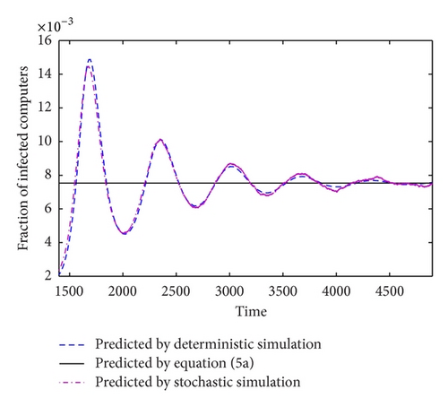
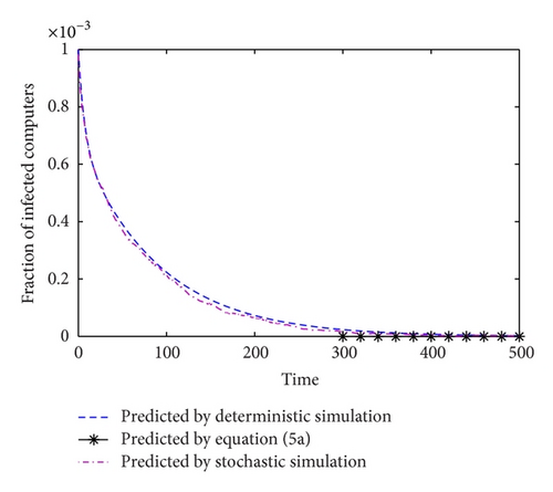
To validate the accuracy of Theorems 1 and 2, we used both deterministic method and stochastic method to simulate the system (3) with N = 1000000, M = 400000, μ₁ = μ₂ = 0.00046, and β₂ = 0.098 and two sets of other variables: (i) β₁ = 0.24, δ₁ = 0.05, and δ₂ = 0.05, where R₀ ≈ 5.98; (ii) β₁ = 0.05, δ₁ = 0.1, and δ₂ = 0.1, where R₀ ≈ 0.85.

As shown in Figure 1, when R₀ > 1, in both deterministic and stochastic simulations, the number of infected computers tends to the theoretical value predicted by (5a) finally, which indicates an endemic state E^*. However, in Figure 2, when R₀ < 1, the steady-state number of I is zero in accordance with the number predicted by disease-free state E₀.

4. Control Strategies

We first give the convergence proof of the numerical method, the improved Euler method, used in the simulation. Let I = (I, R, M_I). Then, we can rewrite the system (3) as $$. Obviously, f is a continuous and differential function in R⁴. Thus, f satisfies the Lipschitz condition and∥f(t, I¹) − f(t, I²)∥ ≤ L∥I¹ − I²∥, where L is a constant.

In this paper, we also use a Monte Carlo algorithm to simulate the propagation of malware [18, 19]. In all simulations given below, we set N = M = 1000000, μ₁ = μ₂ = 0.00046, β₁ = 0.06, β₂ = 2, δ₁ = 0.06, δ₂ = 0.033, α₂ = 0.0001, and λ₂ = 32, where β₁ ≪ β₂ because that malware such as Stuxnet is mainly spreading via removable devices to infect physically isolated machines. The initial numbers of I and M_I are set to 1000 and 0, respectively.

First, we compared three different models with the same parameters: homogeneous model presented in [9] where removable devices are assumed to be used with the same probability on all computers; heterogeneous model presented in [13] where the using rate of removable devices is divided into two rates (using rate on local computers and using rate on the other computers); and the model in this paper. We ran the simulation 100 times and got the average number of infected computers. Figure 3 shows the simulation results.

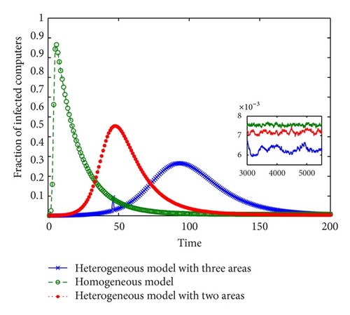
As shown in Figure 3, the model in this paper leads to the lowest infection rate and propagation speed. As it is established under the most reasonable assumptions among three models, its prediction is in accordance with the real propagation process to the most degree. The homogeneous model obtains the highest infection rate and the fastest propagation speed. Although the heterogeneity in removable devices’ using rate is included in the model given in [13], this simplistic division of removable devices’ using rate also leads to a great deviation.

We also simulated various α₁ and λ₁ to gain some insight into the containment of the malware considered in this paper. Figures 4(a) and 4(b) give the simulation results with fixed λ₁ and fixed α₁, respectively.

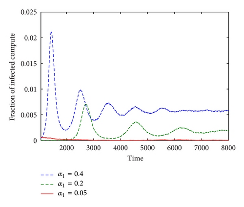
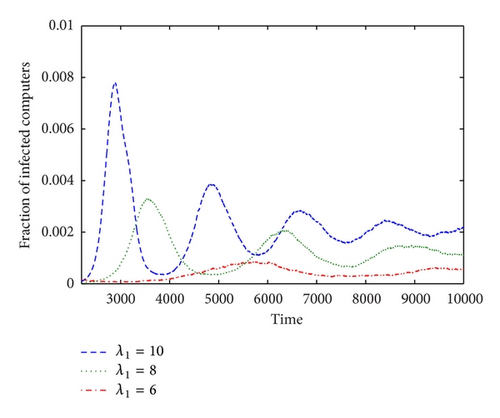
Figures 4(a) and 4(b) show that the radius of neighbour area (λ₁) and the using rate (α₁) in this area have great influences on the propagation of malware. The infection rate and speed decrease rapidly with the decrease of using rate (α₁) or neighbour area’s radius (λ₁). In Figure 4(a) with fixed λ₁(10), the malware dies out directly when α₁ = 0.05, which means an effective countermalware method.

To get the effective countermalware thresholds under various values of λ₁, we further simulated the system (3) and got the values of α₁ below which the malware would die out. Figure 5 plots the simulation results.

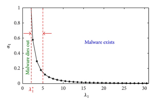
As it is shown in Figure 5, the points in left area can guarantee the extinction of malware. However, the malware can self perpetuate in the right area. The threshold of α₁ decreases with the increase of λ₁ and this decrease is much faster in the area between two arrows ($$). Furthermore, when the radius of neighbour area is less than two times of the radius of local area, corresponding to $$ (=2), the malware will die out no matter what value α₁ is, which gives a promising countermalware threshold.

5. Conclusion

Recently, the researches concerning malware have focused on those pieces malware spreading via removable devices [9–13]. Different from these researches, we present a model with a detailed depiction of the heterogeneity in removable devices’ using rate. This consideration of heterogeneity can lead to an effective countermalware method by controlling the removable devices’ using rate in neighbour area. Furthermore, when α₁ = α₂ = 1, the model presented in this paper corresponds to the model given in [9, 12]; when α₁ = α₂ < 1, it corresponds to the model given in [13]. Thus, the model in this paper is a more general model and can depict the malware’s spreading process more precisely.

Mathematical analysis and stochastic simulations indicate that the dynamics are determined by the value of R₀. Simulation results have also shown that removable devices’ using rate and the radius of neighbour area have great influences on the dynamics of malware. Specifically, we have obtained the thresholds of removable devices’ using rate (α₁) when different values of λ₁ (the radius of neighbour area) are considered, which can guide us in designing effective countermalware method.

In the future, we plan to use real trace data to test our model, especially the special value of removable devices’ using area ($$) and then get the most effective policy to help people in defending their devices and machines against malware.