A worm spread model concerning impulsive control strategy is proposed and analyzed. We prove that there exists a globally attractive virus-free periodic solution when the vaccination rate is larger than θ₁. Moreover, we show that the system is uniformly persistent if the vaccination rate is less than θ₁. Some numerical simulations are also given to illustrate our main results.

1. Introduction

Computer virus is a kind of computer program that can replicate itself and spread from one computer to others including viruses, worms, and trojan horses. Worms use system vulnerability to search and attack computers. As hardware and software technologies develop and computer networks become an essential tool for daily life, worms start to be a major threat. In June 2010, the Belarusian security firm Virus Block Ada discovered deadly Stuxnet worm. The Stuxnet worm is the first known example of a cyber-weapon that is designed not just to steal and manipulate data but to attack a processing system and cause physical damage. The Stuxnet worm is the first cyber-attack of its kind and has infected thousands of computer systems worldwide.

Consequently, the trial on better understanding the worm propagation dynamics is an important matter for improving the safety and reliability in computer systems and networks. Similar to the biological viruses, there are two ways to study this problem: microscopic and macroscopic. Following a macroscopic approach, since [1, 2] took the first step towards modeling the spread behavior of worms, much effort has been done in the area of developing a mathematical model for the worms propagation [3–13]. These models provide a reasonable qualitative understanding of the conditions under which viruses spread much faster than others and why.

In [7], the authors investigated a differential SEIR model by making the following assumptions (Figure 1).

Details are in the caption following the image — **Figure 1**
Open in figure viewer PowerPoint

Original model.

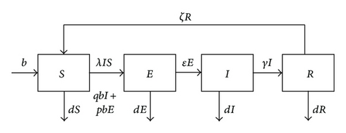
A population size N(t), that is, the total nodes at any time t in the computer network, is partitioned into subclasses of nodes which are susceptible, exposed (infected but not yet infectious), infectious, and recovered with sizes denoted by S(t), E(t), I(t), and R(t), respectively.

One has

()

where b, d, and λ are positive constants and ε, η, γ, ζ are nonnegative constants. The constant b is the recruitment rate of susceptible nodes to the computer network, d is the per capita natural mortality rate (i.e., the crashing of nodes due to the reason other than the attack of worms), ε is the rate constant for nodes leaving the exposed class E for infective class I, γ is the rate constant for nodes leaving the infective class I for recovered class R, η is the disease related death rate (i.e., crashing of nodes due to the attack of worms) in the class I, and ζ is the rate constant for nodes becoming susceptible again after recovering.

In the SEIRS model, the flow is from class S to class E, class E to class I, class I to class R, and again class R to class S. For the vertical transformation, we assume that a fraction p and a fraction q of the new nodes from the exposed and the infectious classes, respectively, are introduced into the exposed class E. Consequently, the birth flux into the exposed class is given by pbE + qbI, and the birth flux into the susceptible class is given by b − pbE − qbI.

As we know, antivirus software is a kind of computer program which can detect and eliminate known worm. There are two common methods to detect worms: using a list of worm signature definition and using a heuristic algorithm to find worm based on common behaviors. It has been observed that it does not always work in detecting a novel worm by using the heuristic algorithm. On the other hand, obviously, it is impossible for antivirus software to find a new worm signature definition on the dated list. So, to keep the antivirus software in high efficiency, it is important to ensure that it is updated. Based on the previous facts, we propose an impulsive system to model the process of periodic installing or updating antivirus software on susceptible computers at fixed time for controlling the spread of worm.

Based on the previous facts, we propose the following assumptions:

(H1)
the antivirus software is installed or updated at time t = kτ(k ∈ N), where τ is the period of the impulsive effect;
(H2)
S computers are successfully vaccinated from S class to R class with rate (0 < θ < 1).

According to the previous assumptions (H1)-(H2) and for the reason of simplicity, we propose the following model (Figure 2):

()

The total population size N(t) can be determined by N(t) = S(t) + E(t) + I(t) + R(t) to form the differential equation

()

which is derived by adding the equations in system (1). Thus the total population size N may vary in time. From (2), we have

()

It follows that

()

The system (2) can be reduced to the equivalent system

()

The initial conditions for (6) are

()

From physical considerations, we discuss system (6) in the closed set

()

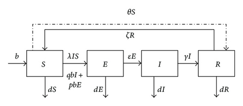
The organization of this paper is as follows. In Section 2, we establish sufficient condition for the local and global attractivity of virus-free periodic solution. The sufficient condition for the permanence of the model is obtained in Section 3. Some numerical simulations are performed in Section 4. In the final section, a brief conclusion is given, and some future research directions are also pointed out.

2. Global Attractivity of Virus-Free Periodic Solution

To prove our main results, we state three lemmas which will be essential to our proofs.

Lemma 1 (see [14].)Consider the following impulsive differential equations:

()

where a > 0, b > 0, and 0 < θ < 1. Then system (9) has a unique positive periodic solution

()

which is globally asymptotically stable; there u^* = a(1 − θ)(1 − e^−bτ)/b(1 − (1 − θ)e^−bτ).

If I(t) ≡ 0, we have the following limit systems:

()

When pb − d − ε < 0, there exists t₁ when t > t₁, lim _t→∞ E(t) = 0. From the third and sixth equations of system (11), we have lim _t→∞ N(t) = b/d. We have the following limit systems:

()

According to Lemma 1, we know that periodic solution of system (12) is of the form

()

and it is globally asymptotically stable, where S^* = ((1 − p)b + (vb/μ))(1 − θ)(e^(μ+v)τ − 1)/(μ + v)(e^(μ+v)τ − 1 + θ).

Theorem 2. Let (S(t), E(t), I(t), N(t)) be any solution of system (6) with initial values S(0⁺) > 0, E(0⁺) > 0, I(0⁺) > 0, and N(0⁺) > 0; then is locally asymptotically stable, provided that pb − d − ε < 0 and R₀ < 1, where

()

Proof. The local stability of virus-free periodic solution may be determined by considering the behaviors of a small amplitude perturbation of the solution. Define , x(t) = E(t), y(t) = I(t), and z(t) = N(t) − b/d, and then the linearized system of system (6) reads as

()

Let Φ(t) be the fundamental solution matrix of system (15), and then Φ(t) must satisfy

()

and Φ(0) = I, the identity matrix. We can easily see that two eigenvalues of the matrix A are −d − ζ and −d, and the other two eigenvalues are determined by the 2 × 2 matrix

. Denote the eigenvalues of B as λ₁, λ₂, and then as pb − d − ε < 0, we have λ₁ + λ₂ = pb − d − ε − r − d − η < 0,

()

Therefore, by the Floquet theorem [15],

is locally asymptotically stable, provided that

()

When R₀ = (1/((d + ε − pb)(γ + d + η)τ − εqbτ))ελ(b/d)[τ + θ(1 − e^(ζ+d)τ)/(ζ + d)(e^(ζ+d)τ − 1 + θ)] ≤ 1, the previous inequality is satisfied for pb − d − ε < 0.

The proof is complete.

Theorem 3. If R₁ ≤ 1, and pb − d − ε < 0 then is globally asymptotically stable for system (11), where

()

Proof. Because e^x − 1 > x, for x > 0, we have

()

By Theorem 2, we know that

is locally asymptotically stable. In the following, we will prove the global attraction of

Let

()

Then

()

Therefore,

is globally asymptotically stable, provided that

()

When R₁ = (1/((d + ε − pb)(γ + d + η)τ − εqbτ))ελ(bτ/d)[1 − θ/(e^(ζ+d)τ − 1 + θ)] ≤ 1, the previous inequality is satisfied.

The proof is complete.

Corollary 4. The virus-free periodic solution of system (6) is globally attractive, if θ > θ₁, where θ₁ = 1 − e^(ζ+d)τ + εbλ(e^(ζ+d)τ − 1)/d[(d + ε − pb)(r + d + η) − εqb].

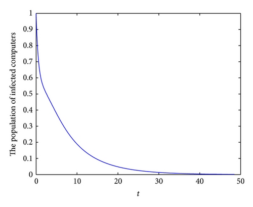
Theorem 2 determines the global attractivity of (6) in Ω for the case R₀ < 1. Its realistic implication is that the infected computers vanish, so the worms are removed from the network. Corollary 4 implies that the computer virus will disappear if the vaccination rate is less than θ₁.

3. Permanence

In this section, we say that the worm is local if the infected population persists above a certain positive level for sufficiently large time. The local of worm can be well captured and studied through the notion of permanence.

Definition 5. System (6) is said to be uniformly persistent if there is an φ > 0 (independent of the initial data) such that every solution (S(t), I(t), R(t), N(t)) with initial conditions (8) of system (6) satisfies

()

Theorem 6. Suppose that R₁ > 1 and pb − d − ε < 0. Then there is a positive constant m_I such that each positive solution (S(t), E(t), I(t), R(t)) of system (6) satisfies I(t) ≥ m_I, for t large enough.

Proof. Now, we will prove that there exist m_I > 0 and a sufficiently large t_p such that I(t) ≥ m_I holds for all t > t_p. Suppose that I(t) < I^* for all t > t₀. From the forth equation of (6), we have

()

From the second equation of (6), we have

()

As pb − d − ε < 0,

()

From the first equation of (6), we have

()

Consider the following comparison system:

()

let

By Lemma 1, we know that there exists t₁ > t₀ such that

()

From the second equation of (6), we have

()

From the third equation of (6); we have

()

Note that R₁ > 1, we have

()

This contradicts I(t) ≤ I^*. Hence, we can claim that for any t₀ > 0, it is impossible that

()

By the claim, we are left to consider two cases. First, I(t) ≥ I^* for t large enough. Second, I(t) oscillates about I^* for t large enough. Obviously, there is nothing to prove for the first case. For the second case, we can choose t₂ > t₁, and ξ > 0 satisfy

()

I(t) is uniformly continuous since the positive solutions of (6) are ultimately bounded, and I(t) is not affected by impulses.

Therefore, it is certain that there exists a η (0 < η < τ, and η is independent of the choice of t₂) such that

()

In this case, we consider the following three possible cases in term of the sizes of η, ξ, and τ.

Case 1. If ξ ≤ η < τ, then it is obvious that I(t) ≥ I^*/2, for t ∈ [t₂, t₂ + ξ].

Case 2. If η < ξ ≤ τ, then from the second equation of system (6), we obtain .

Since I(t₂) = I^*, it is obvious that , for t ∈ [t₂, t₂ + ξ].

Case 3. If η < τ ≤ ξ, it is easy to obtain that I(t) > I^** for t ∈ [t₂, t₂ + τ]. Then, proceeding exactly as the proof for the previous claim, we have that I(t) > I^** for t ∈ [t₂ + τ, t₂ + ξ].

Owing to the randomicity of t₂, we can obtain that there exists such I(t) > m_I holds for all t > t_p.

The proof of Theorem 6 is completed.

Theorem 7. Suppose R₁ > 1. Then system (6) is permanent.

Proof. Let (S(t), E(t), I(t), N(t)) be any solution of system (6). First, from the first equation of system (6), we have

()

Consider the following comparison system:

()

By Lemma 1, we know that for any sufficiently small ε > 0, there exists a t₁ (t₁ is sufficiently large) such that

()

From (31), we have

()

From the third equation of (6), we have

()

It is easy to see that

()

We let

, m_I ≤ I, m_N ≤ N ≤ b/μ, S + I ≤ b/μ}. By Theorem 6 and the previous discussions, we know that the set Ω₀ is a global attractor in Ω, and of course, every solution of system (6) with initial conditions (8) will eventually enter and remain in region Ω₀. Therefore, system (6) is permanent.

The proof of Theorem 7 is completed.

Corollary 8. It follows from Theorem 6 that the system (6) is uniformly persistent, provided that θ < θ₁, where θ₁ = 1 − e^(ζ+d)τ + εbλ(e^(ζ+d)τ − 1)/d[(d + ε − pb)(r + d + η) − εqb].

4. Numerical Simulations

In this section we have performed some numerical simulations to show the geometric impression of our results.

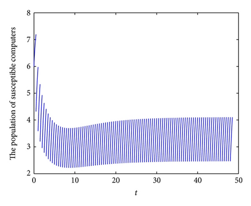
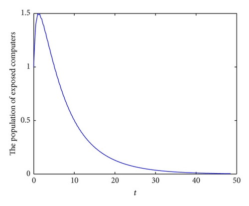
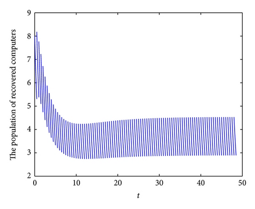
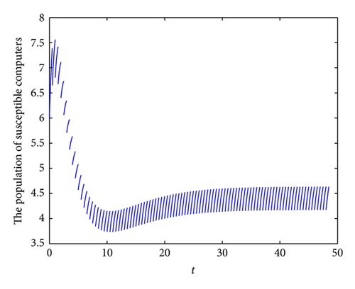
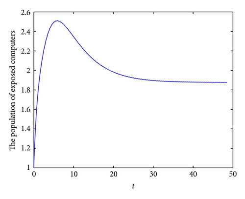
To demonstrate the global attractivity of virus-free periodic solution of system (6), we take following set parameter values: b = 2.1, λ = 0.2, p = 0.1, q = 0.15, d = 0.3, ζ = 0.6, ε = 0.4, γ = 0.6, τ = 0.5, η = 0.3, and θ = 0.4. In this case, we have R₀ = 0.6886 < 1. In Figures 3(a), 3(b), 3(c), and 3(d), we have displayed, respectively, the susceptible, exposed, infected and recovered population of system (6) with initial conditions: S(0) = 6, E(0) = 1, I(0) = 1, and R(0) = 8.

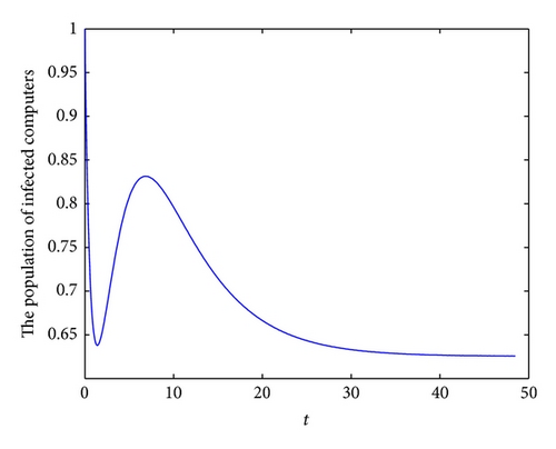
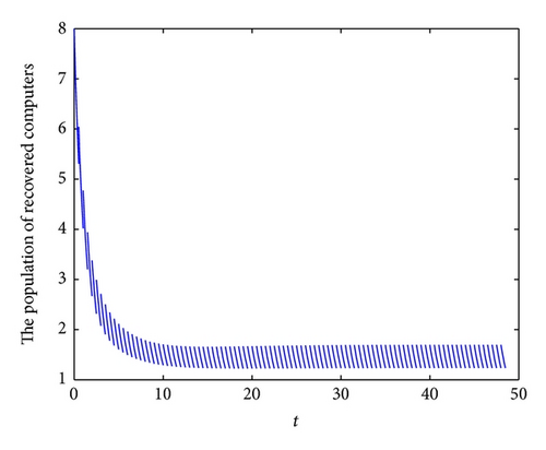
To demonstrate the permanence of system (6), we take the following set parameter values: b = 2.7, λ = 0.2, p = 0.1, q = 0.15, d = 0.3, ζ = 0.6, ε = 0.4, γ = 0.6, τ = 0.5, η = 0.3 and θ = 0.1. In this case, we have R₁ = 1.6496 > 1. In Figures 4(a), 4(b), 4(c), and 4(d), we have displayed, respectively, the susceptible, exposed, infected, and recovered populations of system (6) with initial conditions: S(0) = 6, E(0) = 1, I(0) = 1 and R(0) = 8.

5. Conclusion

We have analyzed the SEIRS model with pulse vaccination and varying total population size. We have shown that R₁ > 1 or θ < θ₁ implies that the worm will be local, whereas R₁ < 1 or θ > θ₁ implies that the worm will fade out. We have also established sufficient condition for the permanence of the model. Our results indicate that a large pulse vaccination rate will lead to eradication of the worm.

References

1 Kephart J. O. and White S. R., Directed-graph epidemiological models of computer viruses, Proceedings of IEEE Symposium on Security and Privacy, 1991, 343–359.
Google Scholar
2 Kephart J. O., White S. R., and Chess D. M., Computers and epidemiology, IEEE Spectrum. (1993) 30, no. 5, 20–26.
10.1109/6.275061
Web of Science® Google Scholar
3 Billings L., Spears W. M., and Schwartz I. B., A unified prediction of computer virus spread in connected networks, Physics Letters A. (2002) 297, no. 3-4, 261–266, https://doi.org/10.1016/S0375-9601(02)00152-4, MR1912464, ZBL0995.68007.
10.1016/S0375-9601(02)00152-4
CAS Web of Science® Google Scholar
4 Han X. and Tan Q., Dynamical behavior of computer virus on Internet, Applied Mathematics and Computation. (2010) 217, no. 6, 2520–2526, https://doi.org/10.1016/j.amc.2010.07.064, MR2733695, ZBL1209.68139.
10.1016/j.amc.2010.07.064
Web of Science® Google Scholar
5 Mishra B. K. and Jha N., Fixed period of temporary immunity after run of anti-malicious software on computer nodes, Applied Mathematics and Computation. (2007) 190, no. 2, 1207–1212, https://doi.org/10.1016/j.amc.2007.02.004.
10.1016/j.amc.2007.02.004
Web of Science® Google Scholar
6 Mishra B. K. and Saini D., Mathematical models on computer viruses, Applied Mathematics and Computation. (2007) 187, no. 2, 929–936, https://doi.org/10.1016/j.amc.2006.09.062, MR2323098, ZBL1120.68041.
10.1016/j.amc.2006.09.062
Web of Science® Google Scholar
7 Mishra B. K. and Pandey S. K., Dynamic model of worms with vertical transmission in computer network, Applied Mathematics and Computation. (2011) 217, no. 21, 8438–8446, https://doi.org/10.1016/j.amc.2011.03.041, MR2802253, ZBL1219.68080.
10.1016/j.amc.2011.03.041
Web of Science® Google Scholar
8 Piqueira J. R. C. and Araujo V. O., A modified epidemiological model for computer viruses, Applied Mathematics and Computation. (2009) 213, no. 2, 355–360, https://doi.org/10.1016/j.amc.2009.03.023, MR2536658, ZBL1185.68133.
10.1016/j.amc.2009.03.023
Web of Science® Google Scholar
9 Piqueira J. R. C., Vasconcelos A. A., Gabriel C. E. C. J., and Araujo V. O., Dynamic models for computer viruses, Computers & Security. (2008) 27, no. 7-8, 355–359, https://doi.org/10.1016/j.cose.2008.07.006.
10.1016/j.cose.2008.07.006
Web of Science® Google Scholar
10 Ren J., Yang X., Yang L.-X., Xu Y., and Yang F., A delayed computer virus propagation model and its dynamics, Chaos, Solitons & Fractals. (2012) 45, no. 1, 74–79, https://doi.org/10.1016/j.chaos.2011.10.003, MR2863589.
10.1016/j.chaos.2011.10.003
Web of Science® Google Scholar
11 Ren J., Yang X., Zhu Q., Yang L. X., and Zhang C., A novel computer virus model and its dynamics, Nonlinear Analysis. (2012) 13, no. 1, 376–384, https://doi.org/10.1016/j.nonrwa.2011.07.048, MR2846848, ZBL1238.34076.
10.1016/j.nonrwa.2011.07.048
Google Scholar
12 Wierman J. C. and Marchette D. J., Modeling computer virus prevalence with a susceptible-infected-susceptible model with reintroduction, Computational Statistics & Data Analysis. (2004) 45, no. 1, 3–23, https://doi.org/10.1016/S0167-9473(03)00113-0, MR2041255.
10.1016/S0167-9473(03)00113-0
Web of Science® Google Scholar
13 Yuan H. and Chen G., Network virus-epidemic model with the point-to-group information propagation, Applied Mathematics and Computation. (2008) 206, no. 1, 357–367, https://doi.org/10.1016/j.amc.2008.09.025, MR2474981, ZBL1162.68404.
10.1016/j.amc.2008.09.025
Web of Science® Google Scholar
14 Gao S., Chen L., and Teng Z., Impulsive vaccination of an SEIRS model with time delay and varying total population size, Bulletin of Mathematical Biology. (2007) 69, no. 1, 731–745, https://doi.org/10.1007/s11538-006-9149-x.
10.1007/s11538-006-9149-x
PubMed Web of Science® Google Scholar
15 Shi R. and Chen L., Stage-structured impulsive SI model for pest management, Discrete Dynamics in Nature and Society. (2007) 11, 97608, https://doi.org/10.1155/2007/97608, MR2375478, ZBL1146.37368.
10.1155/2007/97608
Web of Science® Google Scholar

Citing Literature

All articles

An Impulse Dynamic Model for Computer Worms

Abstract

1. Introduction

2. Global Attractivity of Virus-Free Periodic Solution

3. Permanence

4. Numerical Simulations

5. Conclusion

References

Citing Literature

Figures

References

Information

About Wiley Online Library

Help & Support

Opportunities

Connect with Wiley

An Impulse Dynamic Model for Computer Worms

Abstract

1. Introduction

2. Global Attractivity of Virus-Free Periodic Solution

3. Permanence

4. Numerical Simulations

5. Conclusion

References

Citing Literature

Figures

References

Related

Information