Volume 2013, Issue 1 282593

Research Article

Open Access

Semi-Idealized Study on Estimation of Partly and Fully Space Varying Open Boundary Conditions for Tidal Models

Jicai Zhang,

Corresponding Author

Jicai Zhang

[email protected]

Institute of Physical Oceanography, Ocean College, Zhejiang University, Hangzhou 310058, China zju.edu.cn

MOE Key Laboratory of Coast and Island Development, Nanjing University, Nanjing 210093, China nju.edu.cn

Search for more papers by this author

Haibo Chen,

Haibo Chen

Laboratory of Physical Oceanography, Ocean University of China, Qingdao 266100, China ouc.edu.cn

China Offshore Environmental Services Ltd., Qingdao 266061, China

Search for more papers by this author

Jicai Zhang,

Corresponding Author

Jicai Zhang

[email protected]

Institute of Physical Oceanography, Ocean College, Zhejiang University, Hangzhou 310058, China zju.edu.cn

MOE Key Laboratory of Coast and Island Development, Nanjing University, Nanjing 210093, China nju.edu.cn

Search for more papers by this author

Haibo Chen,

Haibo Chen

Laboratory of Physical Oceanography, Ocean University of China, Qingdao 266100, China ouc.edu.cn

China Offshore Environmental Services Ltd., Qingdao 266061, China

Search for more papers by this author

First published: 22 October 2013

https://doi.org/10.1155/2013/282593

Citations: 3

Academic Editor: Rasajit Bera

Share a link

Email
Wechat
Bluesky

Abstract

Two strategies for estimating open boundary conditions (OBCs) with adjoint method are compared by carrying out semi-idealized numerical experiments. In the first strategy, the OBC is assumed to be partly space varying and generated by linearly interpolating the values at selected feature points. The advantage is that the values at feature points are taken as control variables so that the variations of the curves can be reproduced by the minimum number of points. In the second strategy, the OBC is assumed to be fully space varying and the values at every open boundary points are taken as control variables. A series of semi-idealized experiments are carried out to compare the effectiveness of two inversion strategies. The results demonstrate that the inversion effect is in inverse proportion to the number of feature points which characterize the spatial complexity of open boundary forcing. The effect of ill-posedness of inverse problem will be amplified if the observations contain noises. The parameter estimation problems with more control variables will be much more sensitive to data noises, and the negative effects of noises can be restricted by reducing the number of control variables. This work provides a concrete evidence that ill-posedness of inverse problem can generate wrong parameter inversion results and produce an unreal “good data fitting.”

1. Introduction

The tides and tidal currents are the basic motion forms of ocean water and play an important role in the research on other processes, such as the storm surge, the circulation and the estuarine dynamics [1, 2]. For tidal models, open boundary conditions (OBCs) are one of the most important parameters, which are determined by the physics of tides and tidal currents. Therefore, how to obtain reasonable and accurate OBCs for regional tidal models has been a subject of ongoing research. Data assimilation methods have been commonly used to optimize the open boundary conditions [3–7].

Data assimilation methods, especially the complex ones like four-dimensional variational (4DVAR), are developed on the base of rigorous mathematical theories, such as inverse problem theory and optimal control theory. The ultimate purpose of applying data assimilation method is to reduce the data misfit between model results and various observations, by either improving the models or dynamically interpolating the observations. Among all the data assimilation methods, the 4DVAR is one of the most effective and powerful approaches. It is based on the optimal control methods and perturbation theory [8, 9]. This technique allows us to retrieve an optimal data for a given model from heterogeneous observation fields [9]. It is an advanced data assimilation method which involves the adjoint method and has the advantage of directly assimilating various observations distributed in time and space into numerical models while maintaining dynamical and physical consistency with the model. The adjoint method is a powerful tool for parameter estimation. Navon [10] presented an important overview on the state of the art of parameter estimation in meteorology and oceanography in view of application of 4DVAR data assimilation techniques to inverse parameter estimation problems. Zhang and Lu [7] studied the parameter estimation problems with a three-dimensional tidal model with 4DVAR and also summarized relative works. More recently, Kazantsev [9] briefly revealed the history of data assimilation starting from Lorenz’s pioneering work and then deeply studied the sensitivity of a shallow-water model to parameters by applying adjoint based technique.

For parameter estimation problems, it is of great importance to reasonably reduce the number of spatially varying control variables because of the ill-posedness of inverse problem. As noted by Yeh in the work of ground water flow parameter estimation, the inverse or parameter estimation problem is often ill-posed and beset by instability and nonuniqueness, particularly if one seeks parameters distributed in space and time domain [11]. The same viewpoint has been put forward by references [12–16]. Consequently, how to reduce the number of parameters to be estimated became an important aspect needing to draw attention to [13–17]. In this work two strategies for inverting the open boundary conditions with adjoint method are compared by carrying out semi-idealized numerical experiments. In the first strategy, the OBC is assumed to be partly space varying and generated by linearly interpolating the values at selected feature points. The feature points are selected by calculating the second-order derivatives of discrete curves and the values at selected feature points are taken as control variables to be estimated. The advantage is that most of the variations of the curves can be reproduced by the minimum number of points. In the second strategy, the OBC is assumed to be fully space varying and the values at every open boundary points are taken as control variables.

This paper is organized as follows. The 2D tidal model with adjoint is briefly described in Section 2. The two inversion strategies are developed in Section 3. A series of semi-idealized numerical experiments are carried out and the results are analyzed and discussed in Section 4. Conclusions in Section 5 complete the paper.

2. The Adjoint Tidal Model

2.1. The 2D Tidal Model

The governing equations for the tides used in the present study are the vertically integrated equations of continuity and momentum:

()

where t is time; λ and ϕ are the east longitude and north latitude, respectively; ζ is the sea surface elevation above the undisturbed sea level; u and v are the east and north components of fluid velocity, respectively,

is the adjusted height of equilibrium tides; R is the radius of the earth, a = Rcosϕ; f = 2Ωsinϕ, where Ω represents the angular speed of earth rotation; g is the acceleration due to gravity, h is the undisturbed water depth and H = h + ζ denotes the total water depth; A is the coefficient of horizontal eddy viscosity; Δ is the Laplace operator and Δ(u, v) = a⁻¹[a⁻¹∂_λ(∂_λ(u, v)) + R⁻¹∂_ϕ(cosϕ∂_ϕ(u, v))]; F_λ and F_ϕ are east and north components of bottom friction terms, respectively, and their expressions are given in quadratic form:

()

2.2. The Adjoint

The general idea of the adjoint method is described as follows. First, a model is defined by an algorithm and its independent variables such as initial conditions, boundary conditions, and empirical parameters. The cost function which measures the data misfit between the modeling results and observations is then minimized through optimizing the control variables. In detail, the cost function decreases along the opposite direction of the gradients with respect to the control variables, and this gradient is calculated by what has become known as the adjoint model. In order to construct the adjoint equations, the cost function is defined as

()

and the Lagrangian function is defined as

()

where

is the observations of surface elevation; Ω_T,S stands for the whole integration area of time and space; μ, ν, and τ are the adjoint variables (namely, Lagrangian multipliers) of u, v, and ζ, respectively. Based on the theory of Lagrangian multiplier method, we have the following first-order derivates of Lagrangian function with respect to all the model variables:

()

Equations (5b) give the original governing (1) and the adjoint equations can be developed from (5a). In (5c), a and b are the Fourier coefficients along the open boundary and C_Q denotes the bottom friction coefficients. From (5c) we can obtain the optimization formulae of model parameters.

Based on (5a) the adjoint equations can be obtained as

()

where Ψ(i, j) (1 ≤ i ≤ 3,1 ≤ j ≤ 2) is a matrix whose components denote the adjoint terms of bottom friction. The components of Ψ for the quadratic parameterizations are given as

()

The numerical schemes for the forward model and the adjoint model in this section are both based on Lu and Zhang [17] and Zhang et al. [18].

3. Methodology

3.1. Feature Points of a Curve

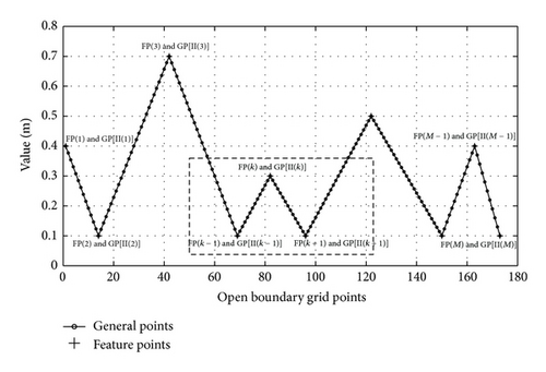
If the values of OBCs are plotted versus the location or index of grid points along open boundaries, they will form a discretized curve. Without loss of generality, the curve can be presented by Figure 1. Assume there are N general (or, computational) points along open boundaries with index of GP(k), k = 1,2, …, N. This type of curve can be approximately linearly expressed by a certain series of points which are defined as feature points in this paper. For the curve shown in Figure 1, one can easily obtain the feature points as indicated by symbol “+.” Assume the number of feature points is M with index of FP(j), j = 1,2, …, M. Further assuming the feature point with index of j is coincident with the general point with index of II(j), we can obtain the following relation: II(1) = 1, II(M) = N, II(j) = k, 2 < k < N − 1.

Details are in the caption following the image — **Figure 1**
Open in figure viewer PowerPoint

Example of discrete curves and their feature points. GP stands for general points and FP indicates feature points.

It is easy to conclude that any general point can be linearly expressed by two adjacent feature points. For example, as shown in Figure 1, an arbitrary general point GP(k) locates between two adjacent feature points FP(j − 1) and FP(j), where II(j − 1) ≤ k ≤ II(j). Through linear interpolation, we can obtain the value of GP(k) as

()

For the whole curve (or the whole boundary), the relation between general points and feature points can be similarly expressed in matrix form as

()

where V_GP and V_FP are both column vectors with dimensions of N and M, respectively, and W_FG is the weighting matrix of linear interpolation with dimensions of N × M. The detailed forms of three matrixes are given as

()

where the nonzero components are the linear interpolation coefficients. Specifically, without loss of generality,

()

Using (9), any general points along open boundaries can be highly approximated through the linear interpolation of selected feature points. It indicates that the OBC identification problem can be transformed to seek the values of a few selected feature points, which reduces the number of control variables.

3.2. Selection of Feature Points for Periodic Tidal Open Boundary

Along a certain open boundary, we also assume that there are N general grid points. The height of water level ζ at the nth time step is given by

()

where GP(k) stands for the general points of open boundaries and 1 ⩽ k ⩽ N, ω is the frequency of M₂ constituent, a_GP(k) and b_GP(k) are the Fourier coefficients at GP(k), Δt is the time step of computation.

For regional tidal models the values of a_GP(k) and b_GP(k) can be obtained from large scale numerical models. It should be noted a_GP(k) and b_GP(k) are space dependent, and therefore the variations of their values versus the grids along the open boundary will constitute two curves (curve_a and curve_b) similar to the one shown in Figure 1. The feature points for this type of curve can be selected by computing the second-order differential of each general point. The detailed selection procedures are given as follows.

(1)
Suppose the absolute values of second-order differentials of general points GP(k) are SD_a(k) for curve_a and SD_b(k) for curve_b, respectively. For the general points locating in the middle of curve_a and curve_b, that is, 2 ⩽ k ⩽ N − 1, SD_a(k) and SD_b(k) can be computed as
()
where Δd is the size of computation grids and equals Δx or Δy according to the direction of open boundaries (Δx for west-east direction and Δy for north-south direction).
(2)
Further define that the “maximum second-order differential” for point GP(k) is SD(k). The value of SD(k) is calculated as
()
(3)
Define a threshold value of SD(k), 2 ⩽ k ⩽ N − 1, to be T_SD. The points with larger values of SD(k) than T_SD are selected as feature points. The value of T_SD is problem dependent and should be determined according to the specific requirement on the number of control variables.
(4)
It is easy to understand that the first and the last general points GP(1) and GP(N) are automatically selected as feature points indexed as FP(1) and FP(M).

3.3. Inversion Strategies and Gradients

In this work two strategies for inverting the open boundary conditions with adjoint method are compared by carrying out semi-idealized numerical experiments. In the first strategy the open boundary curves are assumed to be partly space varying and are generated by linearly interpolating the values at feature points. The feature points are selected by calculating the second-order derivatives of discrete curves and the values at selected feature points are taken as control variables to be estimated. The advantage is that most of the variations of the curves can be reproduced by the minimum number of points. In the second strategy, the OBC is assumed to be fully space varying and the values at every open boundary point are taken as control variables.

The Broyden-Fletcher-Goldfarb-Shanno (BFGS) method, which is a quasi-Newton conjugate-gradient algorithm, has been widely used in the unconstrained inverse problems and is famous for its efficiency [19, 20]. The limited-memory BFGS (L-BFGS) algorithm is an adaptation of the BFGS method to large problem. Zou et al. [20] concluded that among the tested quasi-Newton methods, the L-BFGS method had the best performance. In this work L-BFGS method is employed to optimize the control variables, namely, the OBCs. In order to perform inversion with L-BFGS, the gradients of cost function with respect to the control variables in two strategies have to be calculated.

3.3.1. Gradients for Partly Space Varying Inversion Strategy

In the first inversion strategy (partly space varying OBC), feature points for open boundary curves are selected and the OBCs at general points can be linearly interpolated from feature points. Consequently, the gradients of cost function with respect to the Fourier coefficients at feature points aa_FP(j) and bb_FP(j) (aa_j and bb_j for simplicity, 1 ⩽ j ⩽ M) have to be computed in order to optimize the OBCs with L-BFGS. The gradients are deduced from

()

which yields

()

where

()

where μ and ν are the adjoint variables of west-east velocity component u and north-south velocity component v, respectively. The values of μ and ν are computed by running the adjoint model.

3.3.2. Gradients for Fully Space Varying Inversion Strategy

In the second strategy, the OBC is assumed to be fully space varying and the values at every open boundary points (i.e., general points) are taken as control variables. Consequently, the gradients of cost function with respect to the Fourier coefficients at general points aa_GP(k) and bb_GP(k) (aa_k and bb_k for simplicity, 1 ⩽ k ⩽ N) have to be computed. The gradients are deduced from

()

which yields

()

where

can also be computed by using (19).

4. Numerical Experiments and Results Analysis

4.1. Model Settings

The computing area in the present study is the Bohai Sea, the Yellow Sea, and the East China Sea (BYECS), typical marginal shelf seas. The spatial resolution for the model is 1/12^∘ × 1/12^∘. T/P altimeter data and tidal gauge data are assimilated into the tidal model. The bathymetry map of the BYECS, the position of T/P satellite tracks, tidal gauge stations, and the open boundaries are shown in Figure 2. Since the purpose of this paper is to discuss the inversion of OBCs, the bottom friction coefficients are fixed in all the experiments.

The numerical experiments in this work are semi-idealized. Specifically, the coastline, the number, and location of the observations are real. On the contrary, the values of open boundary conditions and observations are artificial. The prescribed open boundary curves are generated by different number of feature points. Apparently, the complexity of open boundary curves is in direct proportion to the number of feature points. For the semi-idealized experiments, only the location of real observations (satellite altimetry and tidal gauge stations) is used and the values of “observations” are obtained by running the dynamic forward model with prescribed open boundary conditions. The advantage of this kind of experiments is that we can obtain a thorough understanding of the “observations.” The “observations” generated by the model can be accurate and we can control the quality of the “observations” by adding artificial error. In addition, because the other factors are real, the conclusions based on these semi-idealized experiments can be more useful for referring.

The semi-idealized numerical experiments are run as follows. First a distribution of artificial Fourier coefficients is prescribed and taken as “true values” of open boundary conditions. Then the forward tidal model is run using the “true values” and the simulation results recorded at grid points of T/P satellite tracks and tidal gauge stations are taken as the “observations.” Having obtained the “observations”, an initial value (taken as zero in this work) of Fourier coefficients is assigned to run the forward model. The differences between simulated values and “observations” will function as the external force to drive the adjoint model. The optimized Fourier coefficients can be obtained through the backward integration of the adjoint equations. The inverse integral time of the adjoint equations is equal to a period of M₂ tide. With the procedures repeated above, the parameters will be optimized continuously and the difference between simulated values and “observations” will be diminished. Meanwhile, the difference between the prescribed and the inverted parameters will also be decreased.

The iteration of optimization will terminate once the following criterion is achieved [21]:

()

where ∥G∥ is the L₂ norm of the gradients of cost function with respect to the control variables (i.e., the Fourier coefficients at feature points), eps is a positive variable that determines the accuracy with which the solution is to be found, and ∥X∥ is the L₂ norm of control variables. Both the values of ∥G∥ and ∥X∥ vary along the iterations. For a correct adjoint model and a reasonable method, ∥G∥ will gradually decrease versus the iteration steps and the inverted values of control variables must gradually approach the prescribed “true values”. When using L-BFGS, the number of corrections used in the BFGS update is taken as 5 (usually between 3 and 7, see Alekseev et al. [19]). In the minimization algorithm, the control variables should be scaled to similar magnitudes on the order of unity because within the optimization algorithm convergence, tolerances, and other criteria are based on an implicit definition of small and large [22]. Zou et al. [20] also proved that the efficiency could be greatly improved by a simple scaling. In twin experiments we use 10 to scale the Fourier coefficients [4].

4.2. Modeling Results

4.2.1. Effects of Complexity of Open Boundary Curves

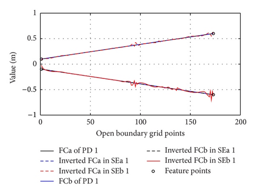
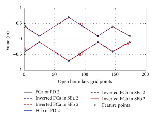
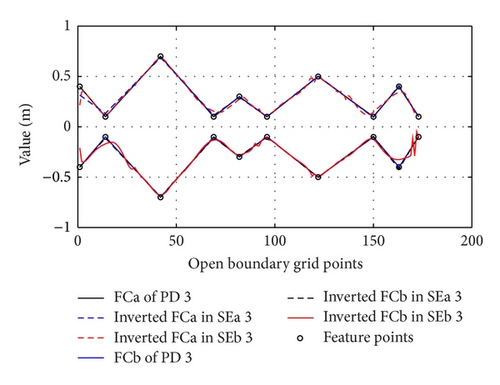
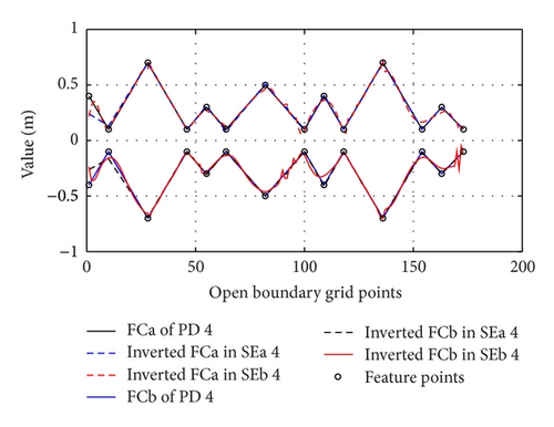
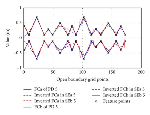
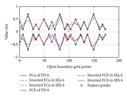
In this section, the semi-idealized experiments (SE) are carried out to calibrate the inversion ability of adjoint model and compare the effectiveness of two strategies developed in Section 3. The prescribed distributions of artificial Fourier coefficients at 173 grid points along the eastern open boundary are inverted. The prescribed distributions (PDs) are designed to be characterized by different numbers of feature points. PDs 1–7 are characterized by 2, 6, 10, 14, 18, 22, and 26 feature points, respectively. The twin experiments are correspondingly indexed with SEa 1–7 for inversion strategy 1 and SEb 1–7 for inversion strategy 2.

The prescribed and inverted distributions of open boundary curves in SEa 1–4 and SEb 1–4 are shown in Figure 3. The prescribed and inverted distributions of open boundary curves in SEa 5-6 and SEb 5-6 are shown in Figure 4. The feature points for prescribed distributions have also been indicated in Figures 3 and 4. Table 1 gives the error statistics for the experiments in this section. The L₂ norm of the gradients of cost function with respect to the control variables versus the iteration steps for the experiments using inversion strategies 1 and 2 are presented in Figures 4(c) and 4(d), respectively. The decrease in data misfit (i.e., cost function) calculated from (3) versus the iteration steps is shown in Figure 5. Note that the values of data misfit and L₂ norm of gradients have been normalized by their values at the first iteration step.

Table 1. Error statistics for SEa 1–7 and SEb 1–7.

Exp.					(m)
Exp.			Before	After	Before	After
Inversion strategy 1
SEa 1	2	0.00	4979.7808	0.0000	0.3500	0.0000
SEa 2	6	0.00	4229.2929	0.0000	0.3332	0.0000
SEa 3	10	0.00	4549.4140	0.1565	0.3055	0.0059
SEa 4	14	0.00	3966.8884	0.1393	0.3121	0.0091
SEa 5	18	0.00	3546.1967	1.0772	0.3014	0.0334
SEa 6	22	0.00	3319.5297	0.7163	0.3066	0.0451
SEa 7	26	0.00	3776.7236	1.2877	0.3124	0.0737

Inversion strategy 2
SEb 1	2	0.00	4979.7808	0.0057	0.3500	0.0101
SEb 2	6	0.00	4229.2929	0.0054	0.3332	0.0125
SEb 3	10	0.00	4549.4140	0.0132	0.3055	0.0152
SEb 4	14	0.00	3966.8884	0.0111	0.3121	0.0194
SEb 5	18	0.00	3546.1967	0.0225	0.3014	0.0472
SEb 6	22	0.00	3319.5297	0.4051	0.3066	0.0662
SEb 7	26	0.00	3776.7236	1.0224	0.3124	0.0783

^aK₁ is the number of feature points for PDs 1–7 prescribed in semi-idealized experiments. K₂ is the value of maximum percentage error. K₃ is the data misfit before and after assimilation. K₄ is the mean absolute difference between prescribed and inverted Fourier coefficients.

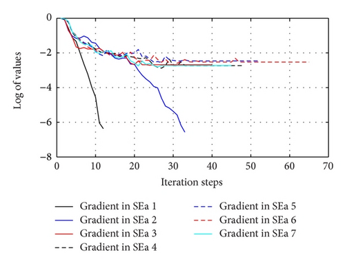
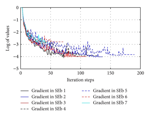
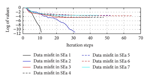
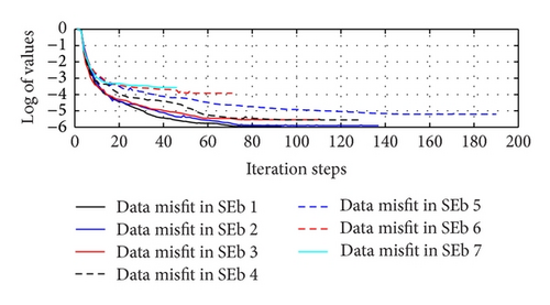
For strategy 1, the values of data misfit can sharply decrease by about 4 orders for all the experiments in about 30 iteration steps. For strategy 2, the values of data misfit can sharply decrease by about 5 orders for SEb 1–5 and by 4 orders for SEb 6-7 in about 60 iteration steps. The decrease in data misfit provides another proof for the inversion ability of the adjoint model and strategies in this work. Correspondingly, the L₂ norms of gradients also decrease by at least 2 orders for inversion strategy 1 and by 3 orders for inversion strategy 2, which demonstrates that the gradients calculated in Section 3.3 can work well with L-BFGS method.

From the decrease in data misfit and gradient it seems as if the effect of inversion strategy 2 is better than that of strategy 1. However, the differences between prescribed and inverted distributions shown in Table 1 indicate that the inversion results of strategy 1 are much better than those of strategy 2. This inconsistency will be explained in Section 4.3. One can find that the adjoint model combined with inversion strategy 1 can reproduce the prescribed distributions of Fourier coefficients perfectly for SEa 1-2 or almost perfectly for SEa 3-4. For SEa 5-6 the inversion is acceptable but largely deviates from perfection. The major trend of the inversion is quite obvious that the effect of inversion is in inverse proportion to the number of feature points which characterizes the complexity of open boundary curves. The inverted open boundary curves shown in Figures 3 and 4 also prove that the inversion using strategy 1 is better than that using strategy 2.

4.2.2. Effects of Data Noises

As we know, the real observations either from satellite altimetry or from tidal gauge stations contain errors (or noises). In this section the effects of the noises are studied. To do this, we replace each “observation” by , where are uniform random numbers lying in [−1,1] and p is a factor determining the maximum percentage error. The maximum percentage errors for each prescribed distribution (PDs 1–7) are assigned to 5%, 10%, 15%, and 20%. The corresponding inversion experiments are then indexed with SE_x i.1, SE_x i.2, SE_x i.3, and SE_x i.4, respectively, where 1 ⩽ i ⩽ 7 and x = a or b. The error statistics for the experiments with P values of 5%, 10%, 15%, and 20% are exhibited in Tables 2, 3, 4, and 5, respectively. The figures are omitted because they are similar to those in Section 4.2.1.

Table 2. Error statistics for SEa 1.1–7.1 and SEb 1.1–7.1.

Exp.					(m)
Exp.			Before	After	Before	After
Inversion strategy 1
SEa 1.1	2	0.05	5060.1284	4.3569	0.3500	0.0011
SEa 2.1	6	0.05	4306.6660	3.5968	0.3332	0.0007
SEa 3.1	10	0.05	4600.6445	3.9834	0.3055	0.0082
SEa 4.1	14	0.05	4019.1911	3.2996	0.3121	0.0093
SEa 5.1	18	0.05	3614.2876	4.0757	0.3014	0.0443
SEa 6.1	22	0.05	3370.5825	3.4881	0.3066	0.0491
SEa 7.1	26	0.05	3838.0024	4.3227	0.3124	0.0740

Inversion strategy 2
SEb 1.1	2	0.05	5060.1284	4.2224	0.3500	0.0238
SEb 2.1	6	0.05	4306.6660	3.4525	0.3332	0.0250
SEb 3.1	10	0.05	4600.6445	3.6353	0.3055	0.0332
SEb 4.1	14	0.05	4019.1911	3.0429	0.3121	0.0337
SEb 5.1	18	0.05	3614.2876	3.0501	0.3014	0.0482
SEb 6.1	22	0.05	3370.5825	2.7539	0.3066	0.0736
SEb 7.1	26	0.05	3838.0024	3.2047	0.3124	0.0833

^aK₁ is the number of feature points for PDs 1–7 prescribed in semi-idealized experiments. K₂ is the value of maximum percentage error. K₃ is the data misfit before and after assimilation. K₄ is the mean absolute difference between prescribed and inverted Fourier coefficients.

Table 3. Error statistics for SEa 1.2–7.2 and SEb 1.2–7.2.

Exp.					(m)
Exp.			Before	After	Before	After
Inversion strategy 1
SEa 1.2	2	0.10	5096.1191	17.4292	0.3500	0.0011
SEa 2.2	6	0.10	4329.9121	14.4080	0.3332	0.0013
SEa 3.2	10	0.10	4621.0439	15.3755	0.3055	0.0115
SEa 4.2	14	0.10	4041.4563	12.8185	0.3121	0.0132
SEa 5.2	18	0.10	3633.7822	13.0238	0.3014	0.0438
SEa 6.2	22	0.10	3388.0535	11.9751	0.3066	0.0540
SEa 7.2	26	0.10	3861.5273	13.5251	0.3124	0.0753

Inversion strategy 2
SEb 1.2	2	0.10	5096.1191	16.7203	0.3500	0.0343
SEb 2.2	6	0.10	4329.9121	13.8206	0.3332	0.0340
SEb 3.2	10	0.10	4621.0439	14.4797	0.3055	0.0456
SEb 4.2	14	0.10	4041.4563	12.1758	0.3121	0.0485
SEb 5.2	18	0.10	3633.7822	11.9745	0.3014	0.0645
SEb 6.2	22	0.10	3388.0535	11.4183	0.3066	0.0846
SEb 7.2	26	0.10	3861.5273	12.1905	0.3124	0.0902

^aK₁ is the number of feature points for PDs 1–7 prescribed in semi-idealized experiments. K₂ is the value of maximum percentage error. K₃ is the data misfit before and after assimilation. K₄ is the mean absolute difference between prescribed and inverted Fourier coefficients.

Table 4. Error statistics for SEa 1.3–7.3 and SEb 1.3–7.3.

Exp.					(m)
Exp.			Before	After	Before	After
Inversion strategy 1
SEa 1.3	2	0.15	5140.9389	39.2166	0.3500	0.0032
SEa 2.3	6	0.15	4360.3886	32.3847	0.3332	0.0018
SEa 3.3	10	0.15	4649.1435	34.2411	0.3055	0.0135
SEa 4.3	14	0.15	4070.1625	28.6868	0.3121	0.0168
SEa 5.3	18	0.15	3659.3095	27.8828	0.3014	0.0446
SEa 6.3	22	0.15	3411.1008	26.0982	0.3066	0.0665
SEa 7.3	26	0.15	3891.3386	28.8848	0.3124	0.0771

Inversion strategy 2
SEb 1.3	2	0.15	5140.9389	37.8465	0.3500	0.0449
SEb 2.3	6	0.15	4360.3886	31.0404	0.3332	0.0430
SEb 3.3	10	0.15	4649.1435	32.1405	0.3055	0.0552
SEb 4.3	14	0.15	4070.1625	27.2928	0.3121	0.0569
SEb 5.3	18	0.15	3659.3095	26.6717	0.3014	0.0700
SEb 6.3	22	0.15	3411.1008	25.1515	0.3066	0.0913
SEb 7.3	26	0.15	3891.3386	27.4780	0.3124	0.0963

^aK₁ is the number of feature points for PDs 1–7 prescribed in semi-idealized experiments. K₂ is the value of maximum percentage error. K₃ is the data misfit before and after assimilation. K₄ is the mean absolute difference between prescribed and inverted Fourier coefficients.

Table 5. Error statistics for SEa 1.4–7.4 and SEb 1.4–7.4.

Exp.					(m)
Exp.			Before	After	Before	After
Inversion strategy 1
SEa 1.4	2	0.20	5194.4404	69.7209	0.3500	0.0043
SEa 2.4	6	0.20	4398.0703	57.5559	0.3332	0.0025
SEa 3.4	10	0.20	4684.9663	61.7102	0.3055	0.0169
SEa 4.4	14	0.20	4105.4169	50.8808	0.3121	0.0207
SEa 5.4	18	0.20	3690.9194	48.2412	0.3014	0.0458
SEa 6.4	22	0.20	3439.8129	45.3626	0.3066	0.0711
SEa 7.4	26	0.20	3927.5261	50.4111	0.3124	0.0792

Inversion strategy 2
SEb 1.4	2	0.20	5194.4404	67.1112	0.3500	0.0562
SEb 2.4	6	0.20	4398.0703	55.1859	0.3332	0.0493
SEb 3.4	10	0.20	4684.9663	57.6774	0.3055	0.0637
SEb 4.4	14	0.20	4105.4169	48.3631	0.3121	0.0644
SEb 5.4	18	0.20	3690.9194	47.1181	0.3014	0.0755
SEb 6.4	22	0.20	3439.8129	43.9302	0.3066	0.0978
SEb 7.4	26	0.20	3927.5261	48.6330	0.3124	0.1011

^aK₁ is the number of feature points for PDs 1–7 prescribed in semi-idealized experiments. K₂ is the value of maximum percentage error. K₃ is the data misfit before and after assimilation. K₄ is the mean absolute difference between prescribed and inverted Fourier coefficients.

One can find the noises in artificial observations will significantly and negatively influence the inversion of open boundary conditions. It is clear that the inversion using strategy 2 is much more sensitive to the noise than that using strategy 1. For example, when the simplest distribution PD 1 is inverted, the difference between prescribed and inverted values will sharply increase from 0.0101 (Table 1) to 0.0238 (Table 2) for strategy 2 even with a small value of error 5%. When P was increased to 20%, the value of this difference is also increased to 0.0562 (Table 5). However, for strategy 1 the values of this difference are just 0.0011, 0.0011, 0.0032 and 0.0043 under P value of 5%, 10%, 15%, and 20%. Similar results can be found from the inversion results of other distributions. This phenomenon indicates that the effect of ill-posedness of inverse problem will be amplified in the conditions that observations contain noises. In addition, the parameter estimation problems with more control variables will be much more sensitive to data noise and the negative effect of noises can be restricted by reducing the number of control variables.

4.3. Discussions

4.3.1. Rationality of the Adjoint Method (Suggested by an Anonymous Reviewer)

The motivation of the present work is to take the open boundary condition as an example to investigate the performance of the adjoint method when applied to ocean modeling and the ill-posedness of relevant inverse problem. The inverse problems in ocean models are often quite complex. The ocean modeling is not just to solve the partial differential equations which might also be solved by some simple methods like the method of characteristics. A reasonable ocean model should also be related to the field observations (satellite altimetry and tidal gauges in this work). In order to realize a more accurate simulation of ocean dynamics, how to organically combine the numerical ocean model with available observations has already become a problem urgent to be solved. Data assimilation methods have been used widely to solve this problem. Among all data assimilation methods, the adjoint data assimilation method is one of the most effective and powerful approaches developed over the past three decades. It is an advanced data assimilation method and has the advantage of directly assimilating various observations distributed in time and space into the numerical model while maintaining dynamical and physical consistency with the model. The adjoint method might be complicated and expensive for some simple problems. However, the inverse problems in ocean modeling are often quite complex in contrast with those simple problems. As is known, one advantage of the numerical method over theoretical analysis lies in the disposal of nonlinear terms. The ocean numerical models are usually strongly nonlinear, increasing the complexity of the relevant inverse problem. Therefore, the increased complexity of the inverse problem makes the adjoint method effective. The adjoint method has been proved to be effective and powerful in ocean and atmosphere problems by many works (see the references listed in Section 1). It has been widely applied to meteorological and oceanographic data assimilation, sensitivity studies, and parameter estimation.

4.3.2. Analysis on Ill-Posedness

From the statistics shown in Tables 1–5, we can find an interesting phenomenon. Define the data misfits after assimilation to be V1_dm for inversion strategy 1 and V2_dm for inversion strategy 2. Further define the differences between prescribed and inverted control variables to be V1_cv for inversion strategy 1 and V2_cv for inversion strategy 2. The values of Vi_cv (i = 1,2) and Vi_dm (i = 1,2) for all the experiments are plotted in Figure 6. We can find V1_dm are larger than or comparable with V2_dm while V1_cv are greatly smaller than V2_cv. Consequently, for all the experiments except SEa 1 and SEa 2, without loss of generality, we can obtain

()

It is easy to understand that small values of Vi_cv (i = 1,2) indicate more accurate control variables, and small values of Vi_dm (i = 1,2) mean small differences between simulated and observed results. In this work, the open boundary conditions are the only parameters for estimation and other parameters are fixed all the time. Instead of formula (23), we should have expected

()

which means a better parameter estimation drives a more accurate simulation. In other words, what we want are small values of V_dm and what we need are small values of V_cv. Formulas (23) and (24) exactly indicate an inconsistency between the effects of parameter estimation and observation restricted data reproduction.

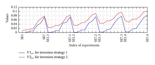
For PDs 1–7 the numbers of feature points are 2, 6, 10, 14, 18, 22, and 26, respectively. It should be noted that at each feature point the Fourier coefficients include a and b. Therefore the numbers of control variables for inversion are doubled, that is, 4, 12, 20, 28, 36, 44, and 52, respectively. There are a total of 35 semi-idealized experiments in this work. Among these experiments, only SEa 1 and SEa 2 can realize a perfect inversion of control variables. Here we define perfect inversion as follows: the data misfit between observed and simulated values can decrease to zero and the difference between prescribed and inverted control variables can also reach a value of zero. With more control variables and larger data noises, the inversion results will not be exactly equal to the prescribed distributions. In the work of Smedstad and O’Brien [12] where the spatially distributed phase speed in an equatorial Pacific Ocean model was estimated, they could not produce the exact values either, even in the condition that perfect observations were available at every grid of the model. Zhang and Lu [4] put forward the similar viewpoint and it also occurs in the parameter estimation of internal tidal model [23–25]. With identical twin experiments, the “observations” are perfect in the sense that they are produced by the model and thus are consistent with the model physics. From the results of this paper and previous works, we can conclude that ill-posedness has happened in other 33 experiments and the effects of ill-posedness will be amplified by increasing the number of control variables and data noises. Formula (23) obtained in this work provides a concrete evidence that ill-posedness of inverse problem can generate poor parameter inversion results while producing an unreal “good data fitting”. For a specific problem, it is necessary and helpful to perform identical semi-idealized experiments in order to find the optimal choices for the number of control variables and inversion strategy.

5. Conclusions

In this work, two strategies for inverting the open boundary conditions with adjoint method are compared by carrying out semi-idealized numerical experiments. In the first strategy, the open boundary curves are assumed to be partly space varying and are generated by linearly interpolating the values at feature points. The feature points are selected by calculating the second-order derivatives of discrete curves and the values at selected feature points are taken as control variables to be estimated. The advantage is that most of the variations of the curves can be reproduced by the minimum number of points. In the second strategy, the OBC is assumed to be fully space varying and the values at every open boundary points are taken as control variables.

A series of semi-idealized experiments are carried out to calibrate the inversion ability of adjoint model and compare the effectiveness of two inversion strategies. The results demonstrate that the effect of inversion is in inverse proportion to the number of feature points which characterize the complexity of open boundary curves. The effect of ill-posedness of inverse problem will be amplified in the conditions that observations contain noises. The parameter estimation problems with more control variables will be much more sensitive to data noises and the negative effects of noises can be restricted by reducing the number of control variables. This work provides a concrete evidence that ill-posedness of inverse problem can generate wrong parameter inversion results while producing an unreal “good data fitting”. For a specific problem, it is necessary and helpful to perform identical semi-idealized experiments in order to find the optimal choices for the number of control variables and inversion strategy.

Acknowledgments

The authors thank Professor Jorge Nocedal at Northwestern University for sharing the source codes of L-BFGS. Partial support for this research was provided by the National Natural Science Foundation of China through Grants 41206001 and 41076006, the Major State Basic Research Development Program of China through Grant 2013CB956500, the Natural Science Foundation of Jiangsu Province through Grant BK2012315, the Priority Academic Program Development of Jiangsu Higher Education Institutions, and the Fundamental Research Funds for the Central Universities 201261006.

References

1 Munk W., Once again: once again-tidal friction, Progress in Oceanography. (1997) 40, no. 1, 7–35, 2-s2.0-0031398016, https://doi.org/10.1016/S0079-6611(97)00021-9.
10.1016/S0079-6611(97)00021-9
Web of Science® Google Scholar
2 Zhang J., Wang P., and Hughes J., EOF analysis of water level variations for microtidal and mangrove-covered Frog Creek system, west-central Florida, Journal of Coastal Research. (2012) 28, no. 5, 1279–1288.
10.2112/JCOASTRES-D-11-00211.1
Web of Science® Google Scholar
3 Zhang A., Wei E., and Parker B. B., Optimal estimation of tidal open boundary conditions using predicted tides and adjoint data assimilation technique, Continental Shelf Research. (2003) 23, no. 11, 1055–1070, 2-s2.0-0242576787, https://doi.org/10.1016/S0278-4343(03)00105-5.
10.1016/S0278-4343(03)00105-5
Web of Science® Google Scholar
4 Zhang J. and Lu X., Inversion of three-dimensional tidal currents in marginal seas by assimilating satellite altimetry, Computer Methods in Applied Mechanics and Engineering. (2010) 199, no. 49–52, 3125–3136, https://doi.org/10.1016/j.cma.2010.06.014, MR2740781, ZBL1225.76300.
10.1016/j.cma.2010.06.014
Web of Science® Google Scholar
5 Strub I. S., Percelay J., Stacey M. T., and Bayen A. M., Inverse estimation of open boundary conditions in tidal channels, Ocean Modelling. (2009) 29, no. 1, 85–93, 2-s2.0-64849103249, https://doi.org/10.1016/j.ocemod.2009.03.002.
10.1016/j.ocemod.2009.03.002
Web of Science® Google Scholar
6 Guo Z., Cao A., and Lu X., Inverse estimation of open boundary conditions in the Bohai Sea, Mathematical Problemsin Engineering. (2012) 2012, 628061, https://doi.org/10.1155/2012/628061.
10.1155/2012/628061
Web of Science® Google Scholar
7 Zhang J. and Lu X., Parameter estimation for a three-dimensional numerical barotropic tidal model with adjoint method, International Journal for Numerical Methods in Fluids. (2008) 57, no. 1, 47–92, https://doi.org/10.1002/fld.1620, MR2402621, ZBL05273009.
10.1002/fld.1620
Web of Science® Google Scholar
8 Marchuk G. I., Formulation of the theory of perturbations for complicated models, Applied Mathematics and Optimization. (1975) 2, no. 1, 1–33, MR0386450, ZBL0324.65053.
10.1007/BF01458193
Web of Science® Google Scholar
9 Kazantsev E., Sensitivity of a shallow-water model to parameters, Nonlinear Analysis: Real World Applications. (2012) 13, no. 3, 1416–1428, https://doi.org/10.1016/j.nonrwa.2011.11.006, MR2863968, ZBL1239.76016.
10.1016/j.nonrwa.2011.11.006
Web of Science® Google Scholar
10 Navon I. M., Practical and theoretical aspects of adjoint parameter estimation and identifiability in meteorology and oceanography, Dynamics of Atmospheres and Oceans. (1998) 27, no. 1–4, 55–79, 2-s2.0-0031944948.
10.1016/S0377-0265(97)00032-8
Web of Science® Google Scholar
11 Yeh W. W.-G., Review of parameter identification procedures in groundwater hydrology: the inverse problem, Water Resources Research. (1986) 22, no. 2, 95–108, 2-s2.0-0022823154.
10.1029/WR022i002p00095
Web of Science® Google Scholar
12 Smedstad O. M. and O′Brien J. J., Variational data assimilation and parameter estimation in an equatorial Pacific ocean model, Progress in Oceanography. (1991) 26, no. 2, 179–241, 2-s2.0-0001119075.
10.1016/0079-6611(91)90002-4
Web of Science® Google Scholar
13 Das S. K. and Lardner R. W., On the estimation of parameters of hydraulic models by assimilation of periodic tidal data, Journal of Geophysical Research. (1991) 96, 15187–15196.
10.1029/91JC01318
Web of Science® Google Scholar
14 Das S. K. and Lardner R. W., Variational parameter estimation for a two-dimensional numerical tidal model, International Journal for Numerical Methods in Fluids. (1992) 15, no. 3, 313–327, https://doi.org/10.1002/fld.1650150305, MR1172865, ZBL0825.76109.
10.1002/fld.1650150305
Web of Science® Google Scholar
15 Ullman D. S. and Wilson R. E., Model parameter estimation from data assimilation modeling: temporal and spatial variability of the bottom drag coefficient, Journal of Geophysical Research C: Oceans. (1998) 103, no. 3, 5531–5549, 2-s2.0-0031780836.
10.1029/97JC03178
Web of Science® Google Scholar
16 Heemink A. W., Mouthaan E. E. A., Roest M. R. T., Vollebregt E. A. H., Robaczewska K. B., and Verlaan M., Inverse 3D shallow water flow modelling of the continental shelf, Continental Shelf Research. (2002) 22, no. 3, 465–484, 2-s2.0-0036186697, https://doi.org/10.1016/S0278-4343(01)00071-1.
10.1016/S0278-4343(01)00071-1
Web of Science® Google Scholar
17 Lu X. and Zhang J., Numerical study on spatially varying bottom friction coefficient of a 2D tidal model with adjoint method, Continental Shelf Research. (2006) 26, no. 16, 1905–1923, 2-s2.0-33748429281, https://doi.org/10.1016/j.csr.2006.06.007.
10.1016/j.csr.2006.06.007
Web of Science® Google Scholar
18 Zhang J., Lu X., Wang P., and Wang Y. P., Study on linear and nonlinear bottom friction parameterizations for regional tidal models using data assimilation, Continental Shelf Research. (2011) 31, no. 6, 555–573, 2-s2.0-79952539172, https://doi.org/10.1016/j.csr.2010.12.011.
10.1016/j.csr.2010.12.011
CAS Web of Science® Google Scholar
19 Alekseev A. K., Navon I. M., and Steward J. L., Comparison of advanced large-scale minimization algorithms for the solution of inverse ill-posed problems, Optimization Methods & Software. (2009) 24, no. 1, 63–87, https://doi.org/10.1080/10556780802370746, MR2489430, ZBL1189.90221.
10.1080/10556780802370746
Web of Science® Google Scholar
20 Zou X., Navon I. M., and Sela J., Control of gravitational oscillations in variational data assimilation, Monthly Weather Review. (1993) 121, no. 1, 272–289, 2-s2.0-0027799822.
10.1175/1520-0493(1993)121<0272:COGOIV>2.0.CO;2
Web of Science® Google Scholar
21 Liu D. C. and Nocedal J., On the limited memory BFGS method for large scale optimization, Mathematical Programming. (1989) 45, no. 3, 503–528, https://doi.org/10.1007/BF01589116, MR1038245, ZBL0696.90048.
10.1007/BF01589116
Web of Science® Google Scholar
22 Navon I. M., Zou X., Derber J., and Sela J., Variational data assimilation with an adiabatic version of the NMC spectral model, Monthly Weather Review. (1992) 120, no. 7, 1433–1446, 2-s2.0-0027073664.
10.1175/1520-0493(1992)120<1433:VDAWAA>2.0.CO;2
Web of Science® Google Scholar
23 Cao A., Chen H., Zhang J., and Lv X., Optimization of open boundary conditions in a 3D internal tidal model with the adjoint method around Hawaii, Abstract and Applied Analysis. (2013) 2013, 11, 950926, https://doi.org/10.1155/2013/950926.
10.1155/2013/950926
Google Scholar
24 Chen H., Miao C., and Lv X., Estimation of open boundary conditions for an internal tidal model with adjoint method: a comparative study on optimization methods, Mathematical Problems in Engineering. (2013) 2013, 12, 802136, https://doi.org/10.1155/2013/802136, MR3035631.
10.1155/2013/802136
Web of Science® Google Scholar
25 Chen H., Cao A., Zhang J., Miao C., and Lv X., Estimation of spatially varying open boundary conditions for a numerical internal tidal model with adjoint method, Mathematics and Computers in Simulation. (2013) https://doi.org/10.1016/j.matcom.2013.08.005.
10.1016/j.matcom.2013.08.005
PubMed Web of Science® Google Scholar

Citing Literature

All articles

Semi-Idealized Study on Estimation of Partly and Fully Space Varying Open Boundary Conditions for Tidal Models

Abstract

1. Introduction