Removing the Correlation Term in Option Pricing Heston Model: Numerical Analysis and Computing
Abstract
This paper deals with the numerical solution of option pricing stochastic volatility model described by a time-dependent, two-dimensional convection-diffusion reaction equation. Firstly, the mixed spatial derivative of the partial differential equation (PDE) is removed by means of the classical technique for reduction of second-order linear partial differential equations to canonical form. An explicit difference scheme with positive coefficients and only five-point computational stencil is constructed. The boundary conditions are adapted to the boundaries of the rhomboid transformed numerical domain. Consistency of the scheme with the PDE is shown and stepsize discretization conditions in order to guarantee stability are established. Illustrative numerical examples are included.
1. Introduction
It is well recognized that the Black-Scholes model, where the prices depend only on the variance of the stock returns, leads to unreliable prices associated with the hypothesis of lognormal distribution of the asset returns and constant volatility. Since 1993, [1] it is known that volatility is a function of both the strike and the expiry date of the derivative security. Empirical evidence suggests that asset price volatility is not constant by variable and stochastic [2].
There are two prominent ways of working around this problem, namely, local volatility models [1] and stochastic volatility models [2–4].
The model proposed by Heston, see [3], [5, chapter 10], takes into account nonlognormal distribution of the assets returns, leverage effect, and important mean-reverting property of volatility and has a closed formula when the parameters are constant [3] or piecewise constant [6].
For constant parameters, Heston [3] uses the method of characteristic functions to derive a closed-form solution involving infinite integrals. When the parameters are piecewise constant in time, one can still derive a recursive closed formula using a PDE method [6] or a Markov argument in combination with affine models [7].
For the case where coefficients are time dependent, the authors in [8] use a small volatility of volatility expansion and Malliavin calculus techniques, to derive approximate analytical solutions. Reliable numerical methods for solving problems (3)–(9) are suitable for both situations, the general time-dependent coefficient case as well as for the constant parameter case, where the closed form proposed solutions require a further numerical treatment.
There are some approaches for the numerical treatment of stochastic volatility models such as sparse wavelet [9], spectral methods [10], and finite-difference methods [11–15].
A feature of the time dependent, two-dimensional convection-diffusion-reaction equation (3) is the presence of a mixed spatial derivative. Dealing with finite-difference methods, this fact involves the existence of negative coefficient terms into the numerical scheme and deteriorates the quality of the numerical solution; see the introduction of [16].
Furthermore, finite difference schemes in the presence of a mixed spatial derivative produces four terms more in the numerical scheme with the corresponding additional computational cost and possible rounding accumulation error.
Both papers [13, 15] construct difference schemes involving the mixed spatial derivative with associated drawbacks. Reference [13] derives a compact finite difference scheme using a nine-point computational stencil. [15] propose three splitting schemes of the alternating direction implicit (ADI) type.
In this paper, we construct explicit finite difference schemes with positive coefficients for solving the Heston model (3)–(9) for the continuously time-dependent coefficient case of the mean reversion rate and long-run variance, after removing the mixed spatial derivative. The organization of the paper is as follows. The problems coming out from negative coefficients arising from the discretization of the diffusion term are not easily remedied [16]; thus, Section 2 addresses the removing of the mixed spatial derivative in (3) by means of the classical technique for the reduction of second-order linear partial differential equations in two variables to canonical form. We also determine the rhomboid nonrectangular numerical domain where the problem is discretized after the transformation. In Section 3, we construct an explicit difference scheme with only a five-points computational stencil. The boundary conditions are adapted to the boundaries of the numerical domain. Section 4 deals with the consistency of the scheme with (3). In Section 5, we study stepsize discretization conditions in order to guarantee the positivity and stability of the numerical scheme. In Section 6, illustrative numerical examples are included.
2. On the Transformation Problem and Its Motivation
Recently, the authors used space-centered forward in time explicit finite difference schemes for the computation and numerical analysis of several one-dimensional option pricing problems [18–20].
Note that if ρ ≠ 0, that is, when variables S and v are correlated, in the last term of the right-hand side of the scheme, (12) involves two terms with negative coefficients because ρ ∈ [−1,1] and σ, vj, and Si are positive. The existence of these terms with negative coefficients does not allow the technique developed in [18–20]. This fact motivates the transformation of problem (3) into an equivalent one where the mixed spatial derivative term disappears.
Remark 1. In the next section, in order to introduce a numerical scheme, we will need to determine a bounded numerical domain.
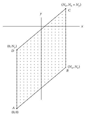
Because of the transformation of the spatial variables (21), a rectangle [S1, S2]×[v1, v2] is transformed into the rhomboid ABCD; see Figure 1, where the sides are described by the following:
Remark 2. For the case |ρ | = 1, fully correlated variables S and v, from (15), the discriminant Δ = 0, and (14) become a parabolic PDE. Following the techniques for reduction to canonical form, an appropriate substitution is x = S; y = v − ρσln S and the transformed equation takes the following form:
3. Numerical Scheme and Boundary Numerical Domain Considerations
Dealing with numerical solutions using finite difference schemes requires the selection of our numerical domain and the transfer of the analytic boundary conditions of the problem to the boundary conditions of the numerical domain avoiding artificial behaviour of the numerical solution [22]. Unlike the classical stepsize discretizations, due to the transformation (21) and Remark 1, we use a discretization of the numerical domain where the stepsize discretizations are related by the slope appearing in (25). Thus, we guarantee that the rhomboid boundary of our numerical domain includes meshpoints of the discretization.
From [23, 24], a suitable bound for the underlying asset variable S is available and generally accepted. In an analogous way, considering an admissible range of the variance v, we can identify a convenient-bounded numerical domain [S1, S2]×[v1, v2] in the Sv plane.
Thus, the rhomboid spatial domain together with its boundary contains (Nx + 1)(Ny + 1) mesh points. See Figure 1.
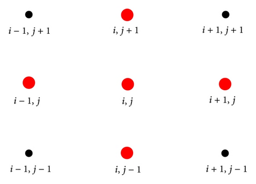
Summarizing, the numerical scheme is expressed by (45) for the internal mesh points, together with the initial condition (47) and the boundary conditions (48)–(51) and (53).
4. Consistency
Summarizing, the following result has been established.
5. Positivity and Stability
We begin this section showing that under suitable relationship between the stepsize discretizations, the coefficients of scheme (45) are nonnegative. This fact together with the positivity of the boundary values will guarantee the positivity of the values of the solution in all time steps at every spatial mesh point.
Lemma 4. Let ha, hb be defined by (81) and (88), respectively, and let h0 = min {ha, hb}. Then, for h < h0 and k satisfying (76), all the coefficients of scheme (45) are nonnegative.
The nonnegativity of the coefficients of scheme (45) is not sufficient to guarantee the positivity of the constructed numerical solution due to the influence on the values at the boundaries of the numerical domain. From (47)–(51), (53), and Lemma 4 it is easy to show the positivity of in all the boundaries of the rhomboid for all n. Hence, the following result has been established.
Theorem 5. Let (xi, yj, τn) be a mesh point in the domain described by Ω (39) with a ≤ xi ≤ b, v1 ≤ mxi − yj ≤ v2. Let be the numerical approximation of W(xi, yj, τn) given by (45) together with the initial condition (47) and the boundary conditions (48)–(51) and (53). Assume that h < h0, where h0 is given by Lemma 4, and k satisfying (76), then for all n, i, j.
The next result is a local discrete maximum principle that guarantees the boundedness of the numerical solution at the internal mesh points of the domain and that will be used below to prove the stability of the scheme.
Lemma 6. Let (i, j) be spatial internal mesh point with 1 ≤ i ≤ Nx − 1; i + 1 ≤ j ≤ Ny + i − 1 and let be the pentaset
Then under conditions of Lemma 4, it follows that
for 0 ≤ n ≤ Nτ − 1.
Proof. From (45), Lemma 4, and using that and that the sum of all the five coefficients of the right-hand side of (45) is one, the result is established.
Definition 7. With previous notation, we say that the solution of the scheme (45), (47)–(51), (53) is ∥·∥1-stable, if for small enough values of h1 = h = Δx, h2 = mΔx and k = Δτ, there is a constant M, independent of n, h, and k, such that
Summarizing, the following result has been established.
Theorem 8. Consider the schemes (45), (47)–(51), (53) in the numerical domain Ω defined by (39) where , and yj ∈ [ma − v2, mb − v1], τn ∈ [0, T]. Let h0 be defined by Lemma 4 and suppose that h = Δx < h0 and k = Δτ is small enough so that condition (76) is satisfied. Then the scheme is ∥·∥1-stable and
6. Examples and Simulations
In this section, we illustrate the good properties of the proposed numerical scheme. Firstly, we consider an example where the closed form solution is available.
Example 1. Consider the European call option for the Heston model (3).
E = 100; T = 1 year; r = 0.01; κ = 2; θ = 0.01; σ = 0.1; ρ = 0.5, v1 = 0.4, and v2 = 0.9.
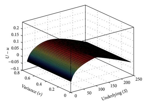
The difference between the closed form solution U and the numerical solution u is shown in Figure 3, by respecting the stability condition (76) and Lemma 4.
The following example shows the variation of the absolute and relative error of the numerical solution in light of the stability and positivity conditions hold at the strike for a given variance for different values of the stepsize discretizations h and k, respectively.
Example 2. Consider the European call option for the Heston mode (3) with data of Example 1 at S = E = 100, v = 0.5. Table 1 shows the behaviour of the error with parameters h and k. Notice that the numerical solution exhibits the expected second order convergence rate in space. Analogously, for fixed h = 0.1 one gets convergence time rate of 0.97. For h = 0.05 the rate is 1.
| k = 0.015 | k = 0.0075 | |||
|---|---|---|---|---|
| h | 0.1 | 0.05 | 0.1 | 0.05 |
| |U − u| | 0.06056 | 0.01594 | 0.03079 | 0.00797 |
| Convergence rate | 1.93 | 1.95 | ||
| Relative error | 2.3 × 10⁻³ | 1.7907 × 10⁻⁴ | 1.2 × 10⁻³ | 8.9537 × 10⁻⁵ |
In the next example, we illustrate the fact that if we do not respect the stability condition, the numerical results are bad and unreliable.
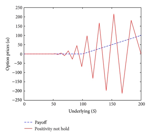
Example 3. Consider the problem of Example 1 at v = 0.9 with h = 0.0082, k = 0.0065, not verifying the stability condition (76). Figure 4 shows that spurious oscillations of the numerical solution appear when the stability condition is broken.
The next example shows the dependence of the option price on both the underlying asset and the variance.
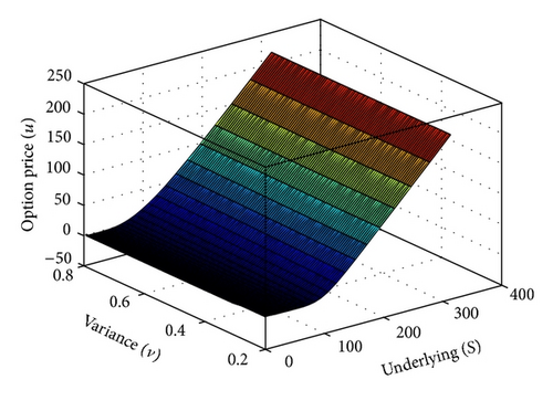
Example 4. Consider the European call option for the Heston model with data.
E = 100; T = 1 year; r = 0.01; κ = 2; θ = 0.01; σ = 0.1; ρ = 0.4 and v1 = 0.2, v2 = 0.9. Figure 5 shows the numerical solution in 3D.
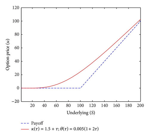
Finally, in the next example, we show the numerical result of a situation with time dependent mean reversion rate κ(τ) and long run variance θ(τ).
Example 5. Consider the European call option for the Heston model with data: E = 100; T = 1 year; r = 0.01; σ = 0.1; ρ = 0.4 and v1 = 0.4, v2 = 0.9 with time-dependent parameters κ(τ) = 1.5 + τ; θ(τ) = 0.005(1 + 2τ). Figure 6 shows the numerical results in this time-dependent case for v = 0.9.
Acknowledgments
This work has been partially supported by the European Union in the FP7-PEOPLE-2012-ITN Program under Grant Agreement no. 304617 (FP7 Marie Curie Action, Project Multi-ITN STRIKE-Novel Methods in Computational Finance) and by the Spanish MEYC Grant DPI2010-20891-C02-01.


