We investigate the statistical inferences and applications of the half exponential power distribution for the first time. The proposed model defined on the nonnegative reals extends the half normal distribution and is more flexible. The characterizations and properties involving moments and some measures based on moments of this distribution are derived. The inference aspects using methods of moment and maximum likelihood are presented. We also study the performance of the estimators using the Monte Carlo simulation. Finally, we illustrate it with two real applications.

1. Introduction

The well-known exponential power (EP) distribution or the generalized normal distribution has the following density function:

(1)

where p > 0 is the shape parameter. This family consists of a wide range of symmetric distributions and allows continuous variation from normality to nonnormality. It includes the normal distribution Z ~ N(0,1) as the special case when p = 2 and the Laplace distribution when p = 1. Nadarajah [1] provided a comprehensive treatment of its mathematical properties.

Its tails can be more platykurtic (p > 2) or more leptokurtic (p < 2) than the normal distribution (p = 2). The distribution has been widely used in the Bayes analysis and robustness studies (see Box and Tiao [2], Genc [3], Goodman and Kotz [4], and Tiao and Lund [5].)

On the other hand, since the most popular models used to describe the lifetime process are defined on nonnegative measurements, which motivate us to take a positive truncation in the model (1) and develop a half exponential power (HEP) distribution. As far as we know, this model has not been previously studied although, we believe, it plays an important role in data analysis. The resulting nonnegative half exponential power distribution generalizes the half normal (HN) distribution, and it is more flexible. In our work, we aim to investigate the statistical features of the nonnegative model and apply them to fit the lifetime data.

The rest of this paper is organized as follows: in Section 2, we present the new distribution and study its properties. Section 3 discusses the inference, moments, and maximum likelihood estimation for the parameters. In Section 4, we discuss a useful technique, a half normal plot with a simulated envelope, to assess the model adequacy. Simulation studies are performed in Section 5. Section 6 gives two illustrative examples and reports the results. Section 7 concludes our work.

2. The Half Exponential Power Distribution

2.1. The Density and Hazard Function

Definition 1. A random variable X has a half exponential power slash distribution if its density function with scale parameter σ > 0 takes

(2)

where σ > 0 and p > 0. We denote it as X ~ HEP(σ, p).

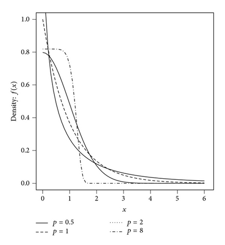
Figure 1(a) displays some plots of the density function of the half exponential power distribution with various parameters.

The cumulative distribution function of the half exponential power distribution X ~ HEP(σ, p) is given as follows. For x ≥ 0,

(3)

where γ(, ) is the lower incomplete gamma function, defined as

The hazard rate function (also known as the failure rate function) of the half exponential power distribution is given by, for x ≥ 0,

(4)

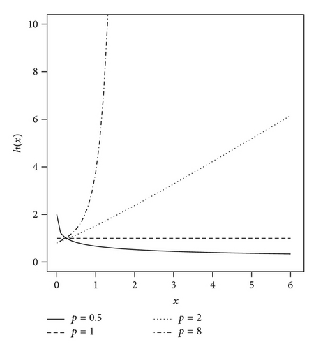
Since Γ(s) − γ(s, x) ~ x^s−1e^−x, as x → ∞, we obtain h(x) ~ x^p−1/σ^p. Therefore, the hazard rate function is increasing for p ≥ 1 and decreasing for 0 < p < 1. Figure 1(b) displays some plots of the hazard rate function of the half exponential power distribution with various parameters.

Details are in the caption following the image — **Figure 1 (a) Density function**
Open in figure viewer PowerPoint

The density and hazard rate functions of HEP(σ, p) for σ = 1.

2.2. Moments and Measures Based on Moments

Proposition 2. Let X ~ HEP(σ, p), for k = 1,2, 3, …; the kth noncentral moments are given by

(5)

The following results are immediate consequences of (5).

Corollary 3. Let X ~ HEP(σ, p). The mean and variance of X are given by

(6)

Corollary 4. Let X ~ HEP(σ, p). The skewness and kurtosis coefficients of X are given by

(7)

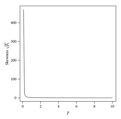
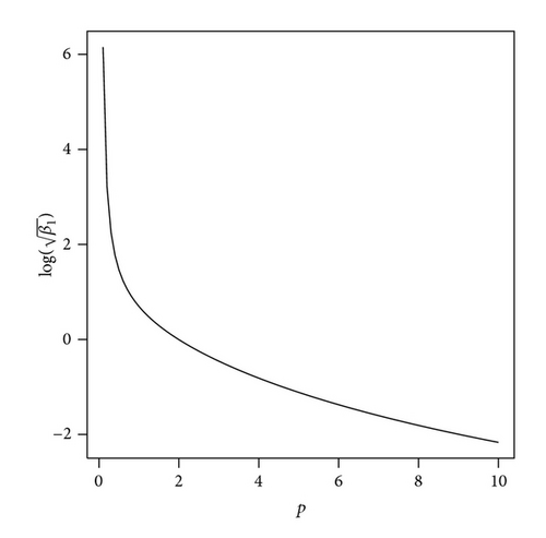
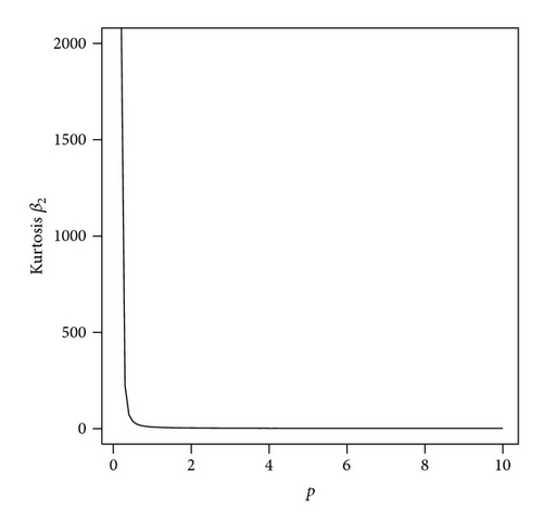
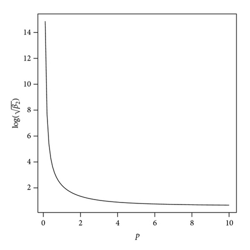
Figure 2 shows the skewness and kurtosis coefficients with various parameters for the HEP model.

3. Inference

3.1. Moment Estimation

Let X₁, X₂, …, X_n be a random sample from the distribution HEP(σ, p). From (5), we have 𝔼X = (p^1/pσ/Γ(1/p))Γ(2/p) and 𝔼X² = (p^2/pσ²/Γ(1/p))Γ(3/p). Replacing 𝔼X and 𝔼X² with the corresponding sample estimators, we obtain the moment equations

(8)

The estimate

is the solution to

(9)

which can be solved numerically. And the estimate

is given by

(10)

It is clear that, for the special case when p is known, estimator

is unbiased and its mean squared error (MSE) is given by

(11)

In the following proposition, we present the asymtotic property of the moment estimators.

Proposition 5. Let X₁, X₂, …, X_n be a random sample of size n from the distribution HEP(σ, p), and let θ = (σ, p); then, if μ₆ = 𝔼X⁶ < ∞ and is the moment estimator of θ, one has

(12)

as n → ∞, where Σ = ({μ_i+j − μ_iμ_j} _ij) and H is given by

(13)

whose entries are given by

(14)

where ψ() is the digamma function defined as the logarithmic derivative of the gamma function, ψ(x) = (d/dx)log Γ(x) = Γ^′(x)/Γ(x).

Remark 6. A consistent estimator for the asymptotic covariance matrix H⁻¹Σ[H⁻¹] ^T can be obtained by replacing parameters with their corresponding moment estimators.

3.2. Maximum Likelihood Estimation

In this section, we consider the maximum likelihood estimation about the parameter θ = (σ, p) of the HEP model defined in (2). The log likelihood for a random sample x₁, x₂, …, x_n is

(15)

By taking the partial derivatives of the log-likelihood function with respect to σ and p, respectively, and equalizing the obtained expressions to zero, the following maximum likelihood estimating equations are obtained:

(16)

In general, there are no explicit solutions for the above maximum likelihood estimating equations. The estimates can be obtained by means of numerical procedures such as the Newton-Raphson method. The program R provides the nonlinear optimization routine optim for solving such problems.

For asymptotic inference of θ = (σ, p), we need the Fisher information matrix I(θ). It is known that its inverse is the asymptotic variance matrix of the maximum likelihood estimators. For the case of a single observation (n = 1), we take the second-order derivatives of the log-likelihood function in (15).

Consider,

(17)

Using the facts

(18)

we can obtain the elements of the Fisher information matrix:

(19)

Proposition 7. Let X₁, X₂, …, X_n be a random sample of size n from the distribution HEP(σ, p), let θ = (σ, p), and is the maximum likelihood estimator of θ, one has

(20)

4. Assessment of Model Adequacy

In this section, we introduce a useful tool, a half normal plot with a simulated envelope which will be used to evaluate the HEP model in Section 6. The advantage of this technique is its ease of interpretation without knowing the distribution of the residuals.

Atkinson [6] proposed this diagnostic plot to detect potential outliers and influential observations in linear regression models. A simulated envelope is added to the plot to aid overall assessment, whereby the observed residuals are expected to lie within the boundary of the envelope if the presumed model has been correctly specified.

The method of simulated envelope and its corresponding transformations have been widely applied in many applications (see Flack and Flores [7], Ferrari and Cribari-Neto [8], da Silva Ferreira et al. [9], and so forth.) The simulated envelope technique compares the observed statistics with those of the data generated from the proposed model. Any sizeble departure of the observed residuals from the simulated quantities may be thought as evidence against the adequacy of the proposed model. Here is the procedure to produce the half normal plot with simulated envelopes.

(1)
Fit the model to the observed data (sample size = n).
(2)
Generate a sample of n observations based on the fitted model.
(3)
Fit the model to the above generated sample and compute the ordered absolute values of the standard residuals.
(4)
Repeat the above steps k times.
(5)
Consider the n sets of the k-ordered statistics; calculate the average, minimum, and maximum values across each set.
(6)
Plot these values together with the ordered residuals from the original data against the half normal scores Φ⁻¹((i + n − 1/8)/(2n + 1/2)).

The minimum and maximum values of the k-ordered statistics constitute a simulated envelope to guide assessment of the model adequacy. Atkinson [6] suggested using k = 19 since there is a 5% chance to detect the largest residual being outside the boundary of the simulated envelope. Moreover, other types of residuals such as deviance or score residual may be used in the procedure. For example, da Silva Ferreira et al. [9] used the Mahalanobis distance to assess their models. The horizontal axis can also show other variables such as index.

5. Simulation Study

In this section, we conduct some simulations and study the properties of the estimators numerically.

We perform a simulation to illustrate the behaviors of the moment and MLE estimators for parameters θ = (σ, p), respectively. The simulation is conducted by the software R. We generate 1000 samples of size n = 100, n = 150, and n = 200 from the HEP(σ, p) distribution for fixed parameters σ and p.

The random numbers can be generated as follows. We first generate random numbers Y from an exponential power distribution with μ = 0, σ, and p, the procedures can be found in Chiodi [10]; then we take the absolute value of the random numbers, X = |Y|. It follows that X ~ HEP(σ, p).

The estimators are computed using the results in Section 3. The empirical means and standard deviations of the estimators are presented in Tables 1 and 2, respectively. The simulation studies show that the parameters are well estimated, and the estimates are asymptotically unbiased. The empirical MSEs decrease as sample size increases as expected. Further, MLEs are more efficient than moment estimators.

Table 1. Empirical means and SD for the moment estimators of σ and p.

σ	p	n = 100		n = 150		n = 200
σ	p	(SD)	(SD)	(SD)	(SD)	(SD)	(SD)
1	1	1.0116 (0.1274)	1.0643 (0.1949)	1.0099 (0.1077)	1.0450 (0.1675)	1.0084 (0.0935)	1.0380 (0.1426)
1	2	1.0046 (0.1014)	2.0544 (0.3443)	0.9989 (0.0816)	2.0369 (0.3167)	1.0034 (0.0745)	2.0484 (0.2869)
1	3	0.9972 (0.0844)	3.0454 (0.4233)	0.9998 (0.0714)	3.0375 (0.4089)	1.0044 (0.0640)	3.0547 (0.3970)

2	1	2.0365 (0.2499)	1.0660 (0.1959)	2.0390 (0.2099)	1.0559 (0.1635)	2.0233 (0.1872)	1.0443 (0.1505)
2	2	2.0090 (0.1983)	2.0726 (0.3453)	2.0111 (0.1710)	2.0541 (0.3117)	2.0014 (0.1424)	2.0372 (0.2814)
2	3	2.0033 (0.1660)	3.0516 (0.4338)	2.0013 (0.1392)	3.0344 (0.4054)	2.0116 (0.1275)	3.0607 (0.3974)

Table 2. Empirical means and SD for the MLE estimators of σ and p.

σ	p	n = 100		n = 150		n = 200
σ	p	(SD)	(SD)	(SD)	(SD)	(SD)	(SD)
1	1	1.0119 (0.1272)	1.0515 (0.2055)	1.0134 (0.1079)	1.0397 (0.1695)	1.0026 (0.0890)	1.0270 (0.1401)
1	2	1.0153 (0.1106)	2.2028 (0.6168)	1.0048 (0.0883)	2.0995 (0.4420)	1.0063 (0.0770)	2.0876 (0.3644)
1	3	1.0193 (0.1102)	3.4735 (1.3164)	1.0099 (0.0816)	3.2477 (0.7742)	1.0068 (0.0736)	3.1542 (0.6405)

2	1	2.0202 (0.2631)	1.0566 (0.2107)	2.0309 (0.2178)	1.0409 (0.1697)	2.0153 (0.1766)	1.0242 (0.1372)
2	2	2.0250 (0.2266)	2.1944 (0.6224)	2.0136 (0.1798)	2.1194 (0.4469)	2.0031 (0.1531)	2.0695 (0.3449)
2	3	2.0332 (0.2235)	3.4523 (1.4561)	2.0241 (0.1682)	3.2700 (0.8226)	2.0218 (0.1432)	3.2229 (0.7221)

6. Real Data Illustration

In this section, we analyze two real datasets to fit with the proposed model. The applications demonstrate that the HEP model fits the data better than the HN model.

6.1. Application 1

The data are the plasma ferritin concentration measurements of 202 athletes collected at the Australian Institute of Sport. This dataset has been studied by several authors (see Azzalini and Dalla Valle [11], Cook and Weisberc [12], and Elal-Olivero et al. [13].)

The descriptive statistics for the dataset are shown in Table 3, where and b₂ are the sample skewness and kurtosis coefficients. Notice that the dataset presents nonnegative measurements.

Table 3. Summary of the plasma ferritin concentration measurements.

Sample size	Mean	Standard deviation		b₂
202	76.88	47.50	1.28	4.42

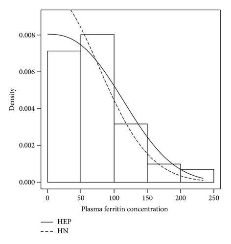
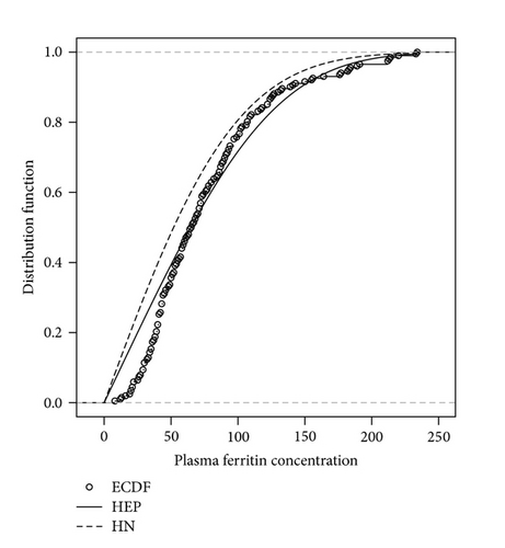
We fit the dataset with the half normal and the half exponential power distribution, respectively, using maximum likelihood method. The MLE estimators are computed using R, and the results are reported in Table 4. The usual Akaike information criterion (AIC) and Bayesian information criterion (BIC) to measure of the goodness of fit are also computed: AIC = 2k − 2logL and BIC = klogn − 2logL, where, k is the number of parameters in the distribution and L is the maximized value of the likelihood function. The results indicate that HEP model has the lower values for the AIC and BIC statistics, and thus it is a better model. Figures 3(a) and 3(b) display the fitted models using the MLE estimates.

Table 4. Maximum likelihood parameter estimates (with (SD)) of the HN and HEP models for the plasma ferritin concentration data.

Model			Log lik.	AIC	BIC
HN	76.9436 (3.0588)	—	−1062.037	2126.074	2129.382
HEP	97.1311 (6.1496)	2.5109 (0.3318)	−1054.739	2113.478	2120.095

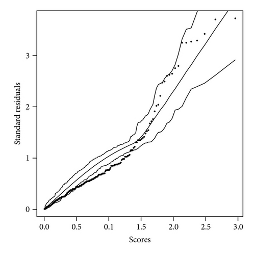
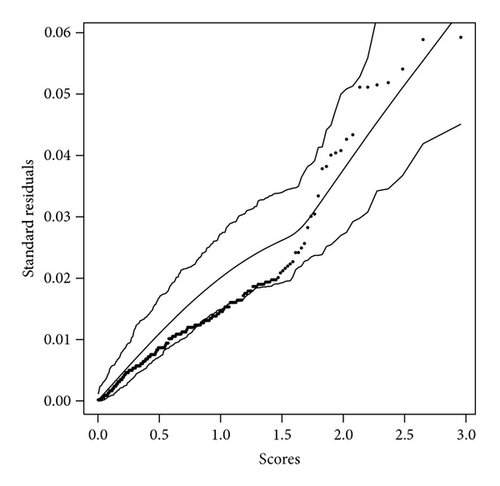
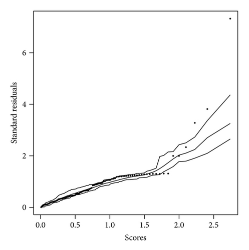
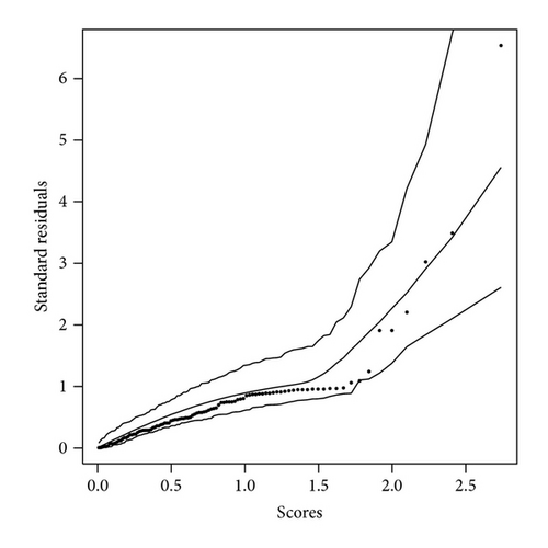
The diagnostic procedure introduced in Section 4 is implemented for both models. The simulated envelope plots are shown in Figures 4(a) and 4(b). Most of the observed residuals are either near or outside the boundary of the envelope, indicating inadequacy of the fitted HN model. On the other hand, the observed residuals corresponding to the HEP model in Figure 4(b) are well within the simulated envelope, indicating that the HEP model provides a better fit to the data.

6.2. Application 2

We consider the stress-rupture dataset and the life of fatigue fracture of Kevlar 49/epoxy that are subject to the pressure at the 90% level. The dataset has been previously studied by Andrews and Herzberg [14], Barlow et al. [15], and Olmos et al. [16].

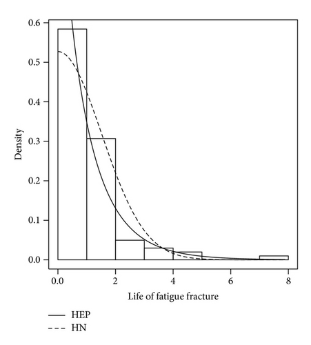
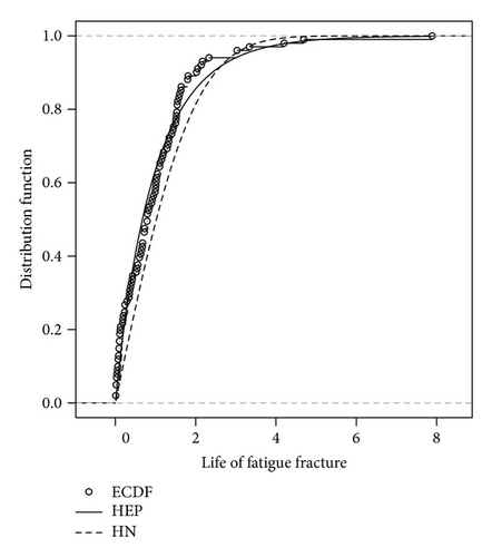
Table 5 summarizes the dataset. This dataset also shows nonnegative asymmetry. Same as before, we fit the dataset with the half normal and the half exponential power distribution, respectively, using maximum likelihood method. The results are reported in Table 6. The AIC and BIC are presented as well, and the results show that HEP model fits better. Figures 5(a) and 5(b) display the fitted models using the MLE estimates.

Table 5. Summaryofthe life of fatigue fracture.

sample size	Mean	Standard deviation		b₂
101	1.025	1.119	3.001	16.709

Table 6. Maximum likelihood parameter estimates (with (SD)) of the HN and HEP models for the life of fatigue fracture data.

Model			Log lik.	AIC	BIC
HN	1.5135 (0.1064)	—	−115.1666	232.3332	234.9483
HEP	0.9689 (0.1298)	0.8815 (0.1677)	−103.2537	210.5074	215.7376

The diagnostic procedure introduced in Section 4 is implemented for both models. The simulated envelope plots are shown in Figures 6(a) and 6(b). The observed residuals corresponding to the HEP model in Figure 6(b) are well within the simulated envelope, indicating that the HEP model provides a better fit to the data.

7. Concluding Remarks

In this paper, we have studied the half exponential power distribution HEP(σ, p) in detail. This nonnegative distribution contains the half normal distribution as its special case. Probabilistic and inferential properties are studied. A simulation is conducted and demonstrates the good performance of the moment and maximum likelihood estimators. We apply the model to two real datasets, illustrating that the proposed model is appropriate and flexible in real applications. There are a number of possible extensions of the current work. Mixture modeling using the proposed distributions is the most natural extension. Other extensions of the current work include a generalization of the distribution to multivariate settings.

Appendix

Proofs of Propositions

Proof of Proposition 2. Consider,

(A.1)

Proof of Proposition 5. This result follows directly by using standard large sample theory for moment estimators, as discussed in Sen and Singer [17].

Proof of Proposition 7. It follows directly by using the large sample theory for maximum likelihood estimators and the Fisher information matrix given above.

References

1 Nadarajah S., A generalized normal distribution, Journal of Applied Statistics. (2005) 32, no. 7, 685–694, 2-s2.0-27644596506, https://doi.org/10.1080/02664760500079464.
Google Scholar
2 Box G. and Tiao G., A further look at robustness via bayes′s theorem, Biometrika. (1962) 49, no. 3-4, 419–432.
Google Scholar
3 Genç A. I., A generalization of the univariate slash by a scale-mixtured exponential power distribution, Communications in Statistics. (2007) 36, no. 5, 937–947, 2-s2.0-34548303608, https://doi.org/10.1080/03610910701539161.
Google Scholar
4 Goodman I. R. and Kotz S., Multivariate θ-generalized normal distributions, Journal of Multivariate Analysis. (1973) 3, no. 2, 204–219, 2-s2.0-0010856550.
Google Scholar
5 Tiao G. and Lund D., The use of olumv estimators in inference robustness studies of the location parameter of a class of symmetric distributions, Journal of the American Statistical Association. (1970) 65, 370–386.
Google Scholar
6 Atkinson A., Plots, Transformations, and Regression: An Introduction to Graphical Methods of Diagnostic Regression Analysis, 1985, Clarendon Press Oxford.
Google Scholar
7 Flack V. F. and Flores R. A., Using simulated envelopes in the evaluation of normal probability plots of regression residuals, Technometrics. (1989) 31, no. 2, 219–225, 2-s2.0-0024657386.
Google Scholar
8 Ferrari S. L. P. and Cribari-Neto F., Beta regression for modelling rates and proportions, Journal of Applied Statistics. (2004) 31, no. 7, 799–815, 2-s2.0-4444357184, https://doi.org/10.1080/0266476042000214501.
Web of Science® Google Scholar
9 da Silva Ferreira C., Bolfarine H., and Lachos V. H., Skew scale mixtures of normal distributions: properties and estimation, Statistical Methodology. (2011) 8, no. 2, 154–171, 2-s2.0-78751705746, https://doi.org/10.1016/j.stamet.2010.09.001.
Google Scholar
10 Chiodi M., Procedures for generating pseudo-random numbers from a normal distribution of order p (P > 1), Statistica Applicata. (1986) 1, 7–26.
Google Scholar
11 Azzalini A. and Dalla Valle A., The multivariate skew-normal distribution, Biometrika. (1996) 83, no. 4, 715–726, 2-s2.0-0001417140.
Google Scholar
12 Cook R. and Weisberc S., An introduction to regression graphic?, Methods. (1994) 17, article 640.
Google Scholar
13 Elal-Olivero D., Olivares-Pacheco J. F., Gómez H. W., and Bolfarine H., A new class of non negative distributions generated by symmetric distributions, Communications in Statistics—Theory and Methods. (2009) 38, no. 7, 993–1008, 2-s2.0-77649316290, https://doi.org/10.1080/03610920802361381.
Google Scholar
14 Andrews D. and Herzberg A., Data: A Collection of Problems from Many Fields for the Student and Research Worker, 1985, 18, Springer, New York, NY, USA.
Google Scholar
15 Barlow R., Toland R., and Freeman T., C. A. Clarotti and D. V. Lindley, A bayesian analysis of the stress-rupture life of kevlar/epoxy spherical pressure vessels, Accelerated Life Testing and Experts Opinions in Reliability, 1988.
Google Scholar
16 Olmos N. M., Varela H., Gómez H. W., and Bolfarine H., An extension of the half-normal distribution, Statistical Papers. (2011) 1–12, 2-s2.0-79959802869, https://doi.org/10.1007/s00362-011-0391-4.
Google Scholar
17 Sen P. and Singer J. M., Large Sample Methods in Statistics: An Introduction with Applications, 1993, Chapman and Hall/CRC.
Google Scholar

Citing Literature

All articles

Statistical Inferences and Applications of the Half Exponential Power Distribution

Abstract

1. Introduction