Electricity is a special energy which is hard to store, so the electricity demand forecasting remains an important problem. Accurate short-term load forecasting (STLF) plays a vital role in power systems because it is the essential part of power system planning and operation, and it is also fundamental in many applications. Considering that an individual forecasting model usually cannot work very well for STLF, a hybrid model based on the seasonal ARIMA model and BP neural network is presented in this paper to improve the forecasting accuracy. Firstly the seasonal ARIMA model is adopted to forecast the electric load demand day ahead; then, by using the residual load demand series obtained in this forecasting process as the original series, the follow-up residual series is forecasted by BP neural network; finally, by summing up the forecasted residual series and the forecasted load demand series got by seasonal ARIMA model, the final load demand forecasting series is obtained. Case studies show that the new strategy is quite useful to improve the accuracy of STLF.

1. Introduction

Load forecasting has always been an essential and important topic for power systems, especially the STLF, which is fundamental in many applications such as providing economic generation, system security, and management and planning [1]. Basic operation functions such as unit commitment, economic dispatch, fuel scheduling, and unit maintenance can be performed more efficiently with an accurate forecasting [2]. However, load forecasting is a difficult task as the load at a given hour is dependent not only on the load at the previous hour but also on the load at the same hour on the previous day and on the load at the same hour on the day with the same denomination in the previous week. The STLF is also difficult to handle due to the nonlinear and random-like behaviors of system load, weather conditions, and variations of social and economic environments, and so forth [3]. So how, to improve the forecasting accuracy is still a difficult and critical problem.

During the past years, a wide variety of techniques have been developed for STLF to improve the forecasting accuracy. For example, in [4], a hybrid fuzzy modeling method by employing the orthogonal least squares method to create the fuzzy model and a constrained optimization algorithm to perform the parameter learning for STLF was presented. Another fuzzy modeling technique was also used for STLF in [5]. Yang and Stenzel proposed a new regression tree method for STLF in [6]; both increment and nonincrement trees were built according to the historical data to provide the data space partition and input variable selections then support vector machine was employed to the samples of regression tree nodes for further fine regression; results of different tree nodes were integrated through weighted average method to obtain the comprehensive forecasting result. Based on state space and Kalman filter approach, a novel time-varying weather and load model for solving the STLF problem was proposed in [7], where time-varying state space model was used to model the load demand on hourly basis while Kalman filter was used recursively to estimate the optimal load forecast parameters for each hour of the day. Considering that STLF was always affected by a variety of nonlinear factors, a mapping function was defined for each factor to identify the nonlinearity in [8]. Several other typical approaches for STLF can be found in [9–12].

The seasonal ARIMA model is frequently employed to forecast data with seasonal item. For instance, Choi et al. [13] used a hybrid SARIMA wavelet transform method for sales forecasting. Egrioglu et al. [14] proposed a hybrid approach based on SARIMA and partial high order bivariate fuzzy time series forecasting model and applied the hybrid model to two real seasonal time series. Besides, Chen and Wang [15] developed a hybrid SARIMA and support vector machines in forecasting the production values of the machinery industry in Taiwan. Considering that the load demand series always contain seasonal item, the seasonal ARIMA model is adopted in this paper.

The BP neural network is a kind of typical feed forward network, through the network structure positive transfer method; using the training function reverse revision network weight matrix and threshold, the BP neural network completes samples training model of the structure and then uses the built training model to complete the treatment of the sample to be measured [16]. The BP neural network model is applied to a wide field of forecasting. As Ke et al. [17] used the genetic algorithm-BP neural network to forecast the electricity power industry loan, Li et al. [18] adopted the BP neural network to the prediction of the mechanical properties of porous NiTi shape memory alloy prepared by thermal explosion reaction. In addition, the BP neural network can also be used for evaluation and classification: Li and Chen [19] utilized the BP neural network algorithm to study the sustainable development evaluation of highway construction project. Bao and Ren showed the wetland landscape classification based on the BP neural network in Dalinor Lake area in [20]. For the BP neural network can approximate the underlying function of the curves to any arbitrary degree of accuracy, this model is also employed to constitute the hybrid model of this paper.

Both ARIMA and BP neural network models have achieved successes in their own linear or nonlinear domains. Though a large number of models have been used to load demand forecasting, more techniques for STLF should be sought to further improve the predictive capability. For this purpose, a hybrid model of combining the seasonal ARIMA model and BP neural network is proposed in this paper. Firstly, the seasonal ARIMA model is adopted to forecast the load demand day ahead then BP neural network is used to forecast the residual series. Finally, by summing up the forecasted residual series and the forecasted load demand, the final load demand is obtained.

The remainder of this paper is organized as follows. Section 2 introduces the combined forecasting model theory. In Section 3, seasonal ARIMA model and BP neural network are presented. In Section 4, a case study of forecasting electricity load of South Australia (SA) State of Australia is demonstrated. Section 5 concludes this paper.

2. The Combined Forecasting Model

The combined forecasting theory states that if there exist M kinds of forecasting models for solving a certain forecasting problem, with properly selected weight coefficients, several forecasting methods’ results can be added up. Assume that y_t (t = 1,2, …, L) is the actual time series data, L is the number of sample points,

is the weight coefficient for the ith forecasting model, the mathematical model of the combined forecasting model can be expressed as follows:

()

where

is the estimated value for ω_i and

is the combined forecasting value.

Determination of the weight coefficients for each individual model is the key step in a construction of a combined forecasting model. This can be achieved by solving an optimization problem which minimizes the absolute error summation for the combined model. This optimization problem can be expressed as follows:

()

The optimization process can be terminated provided that the predefined absolute error summation is reached or the maximum iteration number is reached.

3. The Hybrid Model

3.1. Review of the Seasonal ARIMA Model

Seasonal ARIMA is an extension of autoregressive integrated moving average (ARIMA), which is one of the most common models in time series forecasting analysis. They originated from autoregressive (AR) model which was firstly proposed by Yule in 1972, moving average (MA) model which was firstly proposed by Walker in 1931, and AR and MA combination model autoregressive integrated moving average model (ARMA). Only in sequence where circumstances are stable, ARMA model is effective, but SARIMA and ARIMA do not have such restrictions. Generally speaking, it is assumed that the time series {x_t∣t = 1,2, …, k} has mean zero. A nonseasonal ARIMA model of order (p, d, q) (denoted by ARIMA (p, d, q)) representing the time series can be expressed as follows:

()

where x_t and ε_t are the actual value and random error at time t, respectively, ϕ_t and θ_t are the coefficients, p is the order of autoregressive, q is the order of moving average polynomials, B denotes the backward shift operator, ∇^d = (1 − B) ^d, d is the order of regular differences and ϕ(B) and θ(B) are, respectively, defined as follows

()

Random errors, ε_t, are assumed to be independently and identically distributed with a mean of zero and a constant variance of σ², and the roots of ϕ(x) = 0 and θ(x) = 0 all lie outside the unit circle [21].

Equation (1) entails several important special cases of the ARIMA family of models. If q = 0, then (1) becomes an AR model for order p. When p = 0, the model reduces to an MA model of order q. One central task of ARIMA model building is to determine the appropriate model order (p, q). Similarly, a seasonal model (p, d, q)(P, D, Q) _s can be written as follows (using the second expression):

()

where p and q are the nonseasonal ARMA orders, d is the number of trend differences, X_t is the observation at time t, B is the back-shift operator, ε_t is the residual (an error term at t time period), φ_p(B), θ_q(B) are polynomials in B of order p and q, respectively, P and Q are the seasonal ARMA orders, D is the number of seasonal differences, s is the seasonal period, and Φ_P(B^s), Θ_Q(B^s) are polynomials in B^s of order P and Q, respectively [22].

The SARIMA model formulation includes four steps [23]:

(i)
Identification of the SARIMA (p, d, q)(P,D,Q)_s structure: use autocorrelation function (ACF) and partial autocorrelation function (PACF) to develop the rough function.
(ii)
Estimation of the unknown parameters.
(iii)
Use of goodness-of-fit tests on the estimated residuals.
(iv)
Forecast future outcomes based on the known data.

The steps of this modeling are identification, estimation, availability tests, and forecasting. In the following, we will specifically introduce the four steps. Identification, the appropriate models are determined from all possible models in this stage. The step of identification consists of determining appropriate AR, MA, or ARMA processes and the order of AR, MA, and/or ARMA models. Estimation, in this step parameters are estimated by using ordinary least squares (OLS) and sometimes nonlinear estimation methods. Estimated parameters of AR and MA processes included in ARIMA model should analyze whether they are stationary and invertible or not, respectively. Availability tests, in this stage, it is determined that the estimated ARIMA models are harmonized or not by diagnostic checking. On the other hand, estimated ARIMA model should have to be carried out the assumption that the processes of AR and MA have to be in the unit circle and the assumption of normality. Forecasting, estimated ARIMA models which keep assumptions as expressed above are used in forecasting in this stage.

3.2. Brief Introduction to the Back Propagation (BP) Neural Network

Artificial neural networks (ANN) is a typical kind of intelligent learning algorithm; it is widely used in some practical application, such as pattern classification, function approximation, optimization, forecast, and automation control [24, 25]. In this section, we will introduce the standard multilayer feed-forward neural network (FNN). FNN is a multilayer perception neural network; it is relative to the single perception neural network that can only solve linear separable classification problem. In order to increase the classification ability of the network, the only method is to use the multilayer network. Because the hidden layer neurons are introduced in the multilayer neural network, neural network has better classification and memory ability, so the corresponding learning algorithm becames the focus of research. In 1986, Rumelhart put forward the BP algorithm which solves the learning problems of the multilayer neural network layer implied in the hidden connection weights and gives a complete mathematical deduction. Because BP algorithm overcomes the drawback of the simple perception cannot solve XOR and some other problems, BP algorithm became the main multilayer perception learning algorithm, an important mode of neural network, and widely used.

The BP, one of the most popular techniques in the field of NN, is a kind of supervised learning neural network, the principle behind which involves using the steepest gradient descent method to reach any small approximation. The learning process consists of two parts: forward propagation and back-propagation. When facing the forward propagation, after implicit unit layer processing, information from the input layer to the output layer, the state of each layer neuron affects only the state of next layer neuron. If it is not a desired output in the output layer, then transferred to a back-propagation, the error signal returns along the original neurons connected channel [26]. In the return process, change the neuron connection weights in each layer; this process is iterative, and finally makes the error signal to the permitted range. From that we can see that, in the multilayer feed forward network, there are two signals in circulation: (1) working signal: after the input signal is applied to the working signal, it propagates forward until the actual output signal is produced in the output side, it is the function of inputs and weights. (2) Error signal: the error is the difference between the actual network output and the due output; it propagates back from the output terminal layer by layer [27].

There are three layers contained in BP: input layer, hidden layer, and output layer. Two nodes of each adjacent layer are directly connected, which is called a link. Each link has a weighted value presenting the relational degree between two nodes. Assume that there are n input neurons, m hidden neurons, and one output neuron, the relationship between the output (y_t) and the inputs (y_t−1, y_t−2, …, y_t−n) have the following mathematical representation:

()

We can infer a training process described by the following equations to update these weighted values, which can be divided into two steps.

(i)
Hidden layer stage: the outputs of all neurons in the hidden layer are calculated by the following steps:
()
Here net_j is the activation value of the jth node, y_j is the output of the hidden layer, and f_H is called the activation function of a node, usually a sigmoid function as follows:
()
(ii)
Output stage: the outputs of all neurons in the output layer are given as follows:
()

Here f_o is the activation function, usually a line function. All weights are assigned with random values initially and are modified by the delta rule according to the learning samples traditionally [28].

Hence, the BP model of (1) in fact performs a nonlinear functional mapping from the past observations (y_t−1, y_t−2, …, y_t−n) to the future value y_t that is, y_t = f(y_t−1, y_t−2, …, y_t−n, w) + ε_t, where w is a vector of all parameters and f is a function determined by the network structure and connection weights. Thus, the neural network is equivalent to a nonlinear autoregressive model. Note that expression (7) implies one output node in the output layer which is typically used for one-step-ahead forecasting.

4. Simulation Results

The electric load demand data used for the simulation are sampled from South Australia (SA) State of Australia at half an hour rate, so for one day, 48 load demand data are included. Figure 1 provides the load demand of SA from June 2, 2007 to July 14, 2007.

Details are in the caption following the image — **Figure 1**
Open in figure viewer PowerPoint

Load demand of SA from June 2, 2007 to July 14, 2007.

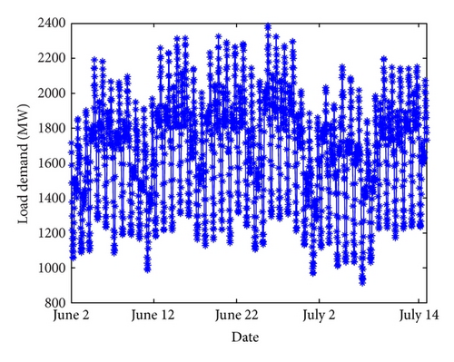
From Figure 1, it can be found that there exists significant similarity in load demand on the same day of each week; in other words seasonal components exist in load demand on the same day of each week. So, the seasonal ARIMA model will be greatly helpful to forecast the load demand day ahead using the historical load demand on the same day several weeks ago. Using the data on June 2, June 9, and June 16 of 2007, the electric load demand on June 23 is forecasted. Then the same way, that is, using the load demand data on the same day of the three sequential weeks to forecast the load demand on the same day of the adjacent week, is adopted to forecast the load demand on June 30, July 7, and July 14. Before the forecasting, values of the parameters should be estimated, obviously, s = 48, other parameters can be estimated by the ACF and PACF figures; values of parameters in forecasting load demand on June 23, June 30, July 7, and July 14 are listed in Table 1. In addition, as an example, ACF and PACF figures in forecasting load demand on June 23 by seasonal ARIMA model are shown in Figures 2 and 3, respectively.

Table 1. Parameters in seasonal ARIMA Model.

Parameters	Forecasting load demand on June 23	Forecasting load demand on June 30	Forecasting load demand on July 7	Forecasting load demand on July 14
p	1	2	1	1
d	1	1	1	1
q	1	1	2	1
P	0	1	0	1
D	1	1	1	1
Q	1	1	0	1

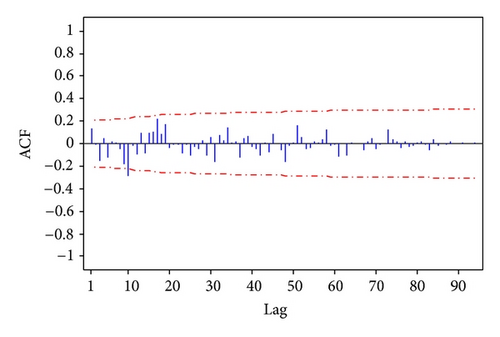
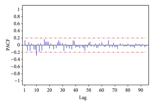
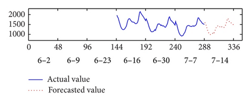
By applying the estimated parameters shown in Table 1 to load demand forecasting, load demand results on June 23, June 30, July 7, and July 14 can be obtained by the seasonal ARIMA models. Forecasted load demand results are shown in Figure 4.

Using these forecasted load demand values, residual errors of load demand series on June 23, June 30, and July 7 will be obtained, as presented in Figure 5. Regarding the residual series as the original data series, the residual series on July 14 can be forecasted. From Figure 4 it can be observed that no significant variation trend can be found in the residual error series; therefore, the BP neural network, which can approximate the underlying function of the curves to any arbitrary degree of accuracy, is employed to forecast the residual error series on July 14. In constructing the BP neural network, one of the most important tasks is training. When for training, the number of nodes in input layer is set as 2, which represent the load demand residual data on June 23 and June 30 at time t, and the corresponding 1-element output will be the residual data on July 7 at the same time, so there are total 48 samples for training. Except for determining the number of nodes in the input layer and output layer, the number of neurons in the hidden layer should also be given to construct the network. For the number of neurons in the hidden layer, we will adopt Hecht-Nelson’s method [29], which is determined as follows:

()

where i is the number of inputs. So the node number in the hidden layer is 5. The structure of the BP neural network is shown in Figure 6.

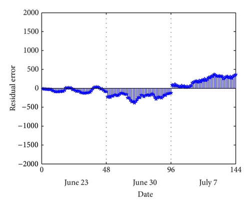
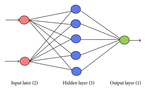
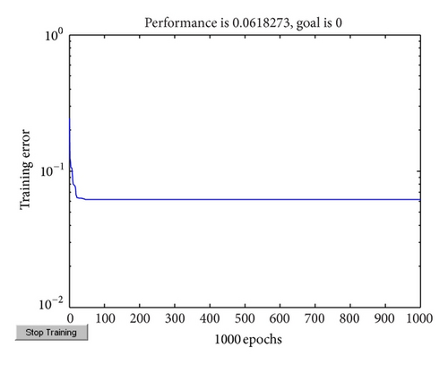
Once the training data and the number of neurons in each layer have been determined, the training process can be conducted. Figure 7 shows the variation of the training error with the epoch number of the BP neural network, where the maximal epoch is 1000.

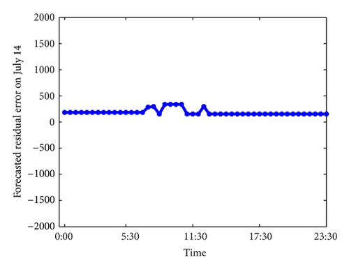
Then the forecasting can be implemented by the trained network. When for forecasting, the residual load demand data on June 30 and July 7 at time t are used for inputs, with which the same time’s load demand on July 14 can be forecasted. Forecasting results are plotted in Figure 8.

Finally, by summing up this forecasted residual series to the forecasted load demand obtained by seasonal ARIMA model, the final load demand can be got, which is shown in Figure 9.

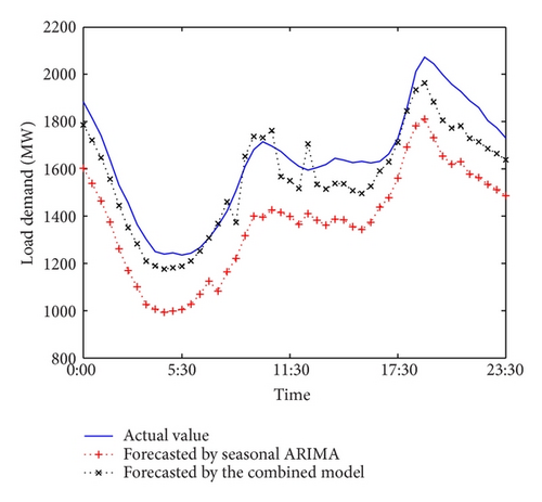
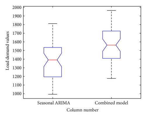
Figure 10 produces whisker plot with two boxes which have lines at the lower, median, and upper quartile values of the load demand forecasted by the single seasonal ARIMA model and the combined model. It can be observed that each of the boxes includes a notch in the position of the median value.

In order to evaluate the performance of the new forecasting strategy, two error measure criteria, that is, the root mean square error (RMSE) and the mean absolute percentage error (MAPE), are used; the forecasting effect is better when the loss function value is smaller. The two error measure criteria are expressed as follows:

()

where x_i and

represent the actual and the forecasted load demand at time i, and the value of N in our simulation is 48. Values of RMSE and MAPE obtained by individual seasonal ARIMA model and by the hybrid model based on seasonal ARIMA and BP neural network are listed in Table 2, and the corresponding bar figure are presented in Figure 11.

Table 2. Comparison of RMSE and MAPE.

Models	RMSE	MAPE (%)
Individual seasonal ARIMA model	260.7376	15.98
Combined model	97.1366	5.13

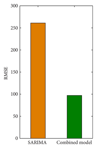
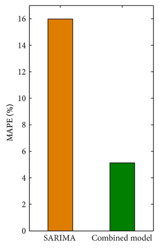
From Table 2 and Figure 11, it can be seen that the value of RMSE varies from 260.7376 in the individual seasonal ARIMA model to 97.1366 in the combined model, while MAPE is reduced from 15.98% to 5.13%. Therefore, the combined model improves the load forecasting accuracy as compared to the individual seasonal ARIMA model.

The performance of the individual seasonal ARIMA model and the combined model in forecasting the load demand is also evaluated by the mean comparison; the comparison result is shown in Figure 12, where group 1, group 2, and group 3 represent the actual load demand, the load demand forecasted by the individual seasonal ARIMA model and the load demand forecasted by the combined model respectively.

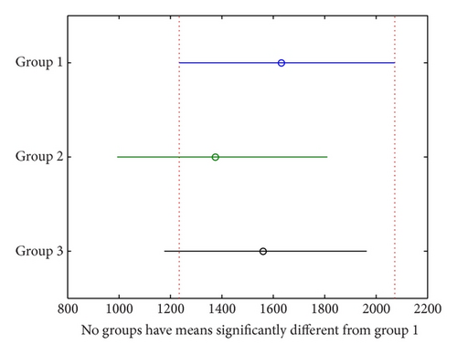
As shown, no groups have means significantly different from group 1, that is, there is no significant difference between the means of the actual load demand and the load demand forecasted by the individual seasonal ARIMA model, as well as the means between the actual load demand and the load demand forecasted by the combined model. However, group 3 occupies more common part with the actual load demand variation range than group 2; thus, the combined model performs better than the individual seasonal ARIMA model in load demand forecasting; that is, the combined model improves the load demand forecasting accuracy as compared to the individual seasonal ARIMA model.

5. Conclusions

Different from usual combined forecasting models, a new strategy for STLF of using combined models is presented in this paper. As many sequences has periodic in real life, so these similar to the SARIMA model which can dig out the periodicity contained in the data is often used to predict and model the time series which have periodic. Secondly, this paper proposed by using the error sequence which SARIMA model predicted to predict the residual series of one day in the future, and by adding the residual series to the load value which got by the BP on the same day to improve the accuracy of the model. But the load prediction value residuals which were obtained by the SARIMA model do not have the same tendency or regularity; therefore, the choice of subsequent residual sequence prediction method should be careful. Considering that the neural network has a good effect for fitting of nonlinear function, this paper uses neural network model which can perfectly reflect the nonlinear relation between the input and output element to predict the subsequent residual sequence and did not use the regression or other model which has clear requirements for the form of the data; this further improves the accuracy of the prediction residuals. Furthermore, according to the characteristics of the model, this paper constructed a validity criterion which can measure the effectiveness of the model. At last, by using this combination method to the electricity load demand forecasting of South Australia, it appears that this combination method has a good effect in improving the prediction precision, because it is relative to the error in 15.98% which was predicted by a single SARIMA model, a hybrid model based on SARIMA, and neural network reduces the load predict error to 5.13%, and the validity criterion increases from 0.8402 to 0.9487. Simulation results demonstrate that the new strategy for STLF is effective in getting satisfying improvement of forecasting accuracy.

Acknowledgments

This work was supported by the Natural Science Foundation of P. R. of China (90912003, 61073193), the Key Science and Technology Foundation of Gansu Province (1102FKDA010), Natural Science Foundation of Gansu Province (1107RJZA188), and the Fundamental Research Funds for the Central Universities (lzujbky-2012-47, lzujbky-2012-48).

References

1 Al-Hamadi H. M. and Soliman S. A., Short-term electric load forecasting based on Kalman filtering algorithm with moving window weather and load model, Electric Power Systems Research. (2004) 68, no. 1, 47–59, 2-s2.0-0142228351, https://doi.org/10.1016/S0378-7796(03)00150-0.
10.1016/S0378-7796(03)00150-0
Web of Science® Google Scholar
2 Senjyu T., Mandal P., Uezato K., and Funabashi T., Next day load curve forecasting using hybrid correction method, IEEE Transactions on Power Systems. (2005) 20, no. 1, 102–109, 2-s2.0-13844320123, https://doi.org/10.1109/TPWRS.2004.831256.
10.1109/TPWRS.2004.831256
Web of Science® Google Scholar
3 Wang B., Tai N. L., Zhai H. Q., Ye J., Zhu J. D., and Qi L. B., A new ARMAX model based on evolutionary algorithm and particle swarm optimization for short-term load forecasting, Electric Power Systems Research. (2008) 78, no. 10, 1679–1685, 2-s2.0-45449091535, https://doi.org/10.1016/j.epsr.2008.02.009.
10.1016/j.epsr.2008.02.009
Web of Science® Google Scholar
4 Mastorocostas P. A., Theocharis J. B., Kiartzis S. J., and Bakirtzis A. G., A hybrid fuzzy modeling method for short-term load forecasting, Mathematics and Computers in Simulation. (2000) 51, no. 3-4, 221–232, 2-s2.0-0000835561, https://doi.org/10.1016/S0378-4754(99)00119-6.
10.1016/S0378-4754(99)00119-6
Web of Science® Google Scholar
5 Papadakis S. E., Theocharis J. B., and Bakirtzis A. G., A load curve based fuzzy modeling technique for short-term load forecasting, Fuzzy Sets and Systems. (2003) 135, no. 2, 279–303, 2-s2.0-0037448873, https://doi.org/10.1016/S0165-0114(02)00211-7, ZBL1031.93011.
10.1016/S0165-0114(02)00211-7
Web of Science® Google Scholar
6 Yang J. F. and Stenzel J., Short-term load forecasting with increment regression tree, Electric Power Systems Research. (2006) 76, no. 9-10, 880–888, 2-s2.0-33645971626, https://doi.org/10.1016/j.epsr.2005.11.007.
10.1016/j.epsr.2005.11.007
Web of Science® Google Scholar
7 Al-Hamadi H. M. and Soliman S. A., Short-term electric load forecasting based on Kalman filtering algorithm with moving window weather and load model, Electric Power Systems Research. (2004) 68, no. 1, 47–59, 2-s2.0-0142228351, https://doi.org/10.1016/S0378-7796(03)00150-0.
10.1016/S0378-7796(03)00150-0
Web of Science® Google Scholar
8 Kang C. Q., Cheng X., Xia Q., Huang Y. H., and Gao F., Novel approach considering load-relative factors in short-term load forecasting, Electric Power Systems Research. (2004) 70, no. 2, 99–107, 2-s2.0-4944233166, https://doi.org/10.1016/j.epsr.2003.11.008.
10.1016/j.epsr.2003.11.008
Web of Science® Google Scholar
9 Fan S., Chen L. N., and Lee W. J., Machine learning based switching model for electricity load forecasting, Energy Conversion and Management. (2008) 49, no. 6, 1331–1344, 2-s2.0-42749089472, https://doi.org/10.1016/j.enconman.2008.01.008.
10.1016/j.enconman.2008.01.008
Web of Science® Google Scholar
10 Srinivasan D., Evolving artificial neural networks for short term load forecasting, Neurocomputing. (1998) 23, no. 1–3, 265–276, 2-s2.0-0032495097, https://doi.org/10.1016/S0925-2312(98)00074-5.
10.1016/S0925-2312(98)00074-5
Web of Science® Google Scholar
11 Chen J. F., Wang W. M., and Huang C. M., Analysis of an adaptive time-series autoregressive moving-average (ARMA) model for short-term load forecasting, Electric Power Systems Research. (1995) 34, no. 3, 187–196, 2-s2.0-0029368511, https://doi.org/10.1016/0378-7796(95)00977-1.
10.1016/0378-7796(95)00977-1
Web of Science® Google Scholar
12 Amaral L. F., Souza R. C., and Stevenson M., A smooth transition periodic autoregressive (STPAR) model for short-term load forecasting, International Journal of Forecasting. (2008) 24, no. 4, 603–615, 2-s2.0-55349088880, https://doi.org/10.1016/j.ijforecast.2008.08.006.
10.1016/j.ijforecast.2008.08.006
Web of Science® Google Scholar
13 Choi T. M., Yu Y., and Au K. F., A hybrid SARIMA wavelet transform method for sales forecasting, Decision Support Systems. (2011) 51, no. 1, 130–140, 2-s2.0-79951508907, https://doi.org/10.1016/j.dss.2010.12.002.
10.1016/j.dss.2010.12.002
Web of Science® Google Scholar
14 Egrioglu E., Aladag C. H., Yolcu U., Basaran M. A., and Uslu V. R., A new hybrid approach based on SARIMA and partial high order bivariate fuzzy time series forecasting model, Expert Systems with Applications. (2009) 36, no. 4, 7424–7434, 2-s2.0-60249083330, https://doi.org/10.1016/j.eswa.2008.09.040.
10.1016/j.eswa.2008.09.040
Web of Science® Google Scholar
15 Chen K. Y. and Wang C. H., A hybrid SARIMA and support vector machines in forecasting the production values of the machinery industry in Taiwan, Expert Systems with Applications. (2007) 32, no. 1, 254–264, 2-s2.0-33748133361, https://doi.org/10.1016/j.eswa.2005.11.027.
10.1016/j.eswa.2005.11.027
Web of Science® Google Scholar
16 Liu H., Chandrasekar V., and Xu G., An adaptive neural network scheme for radar rainfall estimation form WSR-88D observations, Journal of Applied Meteorology. (2001) 40, no. 11, 2038–2050.
10.1175/1520-0450(2001)040<2038:AANNSF>2.0.CO;2
Web of Science® Google Scholar
17 Ke L., Wenyan G., Xiaoliu S., and Zhongfu T., Research on the forecast model of electricity power industry loan based on GA-BP neural network, Energy Procedia. (2012) 14, 1918–1924, https://doi.org/10.1016/j.egypro.2011.12.1188.
10.1016/j.egypro.2011.12.1188
Google Scholar
18 Li Q., Yu J. Y., Mu B. C., and Sun X. D., BP neural network prediction of the mechanical properties of porous NiTi shape memory alloy prepared by thermal explosion reaction, Materials Science and Engineering A. (2006) 419, no. 1-2, 214–217, 2-s2.0-33644908017, https://doi.org/10.1016/j.msea.2005.12.027.
10.1016/j.msea.2005.12.027
Web of Science® Google Scholar
19 Li M. and Chen W., Application of BP neural network algorithm in sustainable development of highway construction projects, Physics Procedia. (2012) 25, 1212–1217, https://doi.org/10.1016/j.phpro.2012.03.222.
10.1016/j.phpro.2012.03.222
Google Scholar
20 Bao Y. H. and Ren J., Wetland landscape classification based on the BP neural network in DaLinor lake area, Procedia Environmental Sciences. (2011) 10, 2360–2366, https://doi.org/10.1016/j.proenv.2011.09.368.
10.1016/j.proenv.2011.09.368
Google Scholar
21 Tseng F. M., Yu H. C., and Tzeng G. H., Combining neural network model with seasonal time series ARIMA model, Technological Forecasting and Social Change. (2002) 69, no. 1, 71–87, 2-s2.0-0036140323, https://doi.org/10.1016/S0040-1625(00)00113-X.
10.1016/S0040-1625(00)00113-X
Web of Science® Google Scholar
22 Lai S. L. and Lu W. L., Impact analysis of September 11 on air travel demand in the USA, Journal of Air Transport Management. (2005) 11, no. 6, 455–458, 2-s2.0-24744442148, https://doi.org/10.1016/j.jairtraman.2005.06.001.
10.1016/j.jairtraman.2005.06.001
Web of Science® Google Scholar
23 Tseng F. M. and Tzeng G. H., A fuzzy seasonal ARIMA model for forecasting, Fuzzy Sets and Systems. (2002) 126, no. 3, 367–376, 2-s2.0-0037117197, https://doi.org/10.1016/S0165-0114(01)00047-1, ZBL1003.62081.
10.1016/S0165-0114(01)00047-1
Web of Science® Google Scholar
24 Mohandes M. A., Rehman S., and Halawani T. O., A neural networks approach for wind speed prediction, Renewable Energy. (1998) 13, no. 3, 345–354, 2-s2.0-0032029065, https://doi.org/10.1016/S0960-1481(98)00001-9.
10.1016/S0960-1481(98)00001-9
Web of Science® Google Scholar
25 Yu L., Wang S., and Lai K. K., Forecasting crude oil price with an EMD-based neural network ensemble learning paradigm, Energy Economics. (2008) 30, no. 5, 2623–2635, 2-s2.0-48049095703, https://doi.org/10.1016/j.eneco.2008.05.003.
10.1016/j.eneco.2008.05.003
Web of Science® Google Scholar
26 Rumelhart D. E., Hinton G. E., and Williams R. J., Learning representations by back-propagating errors, Nature. (1986) 323, no. 6088, 533–536, 2-s2.0-0022471098, https://doi.org/10.1038/323533a0.
10.1038/323533a0
Web of Science® Google Scholar
27 Hippert H. S., Pedreira C. E., and Souza R. C., Neural networks for short-term load forecasting: a review and evaluation, IEEE Transactions on Power Systems. (2001) 16, no. 1, 44–55, 2-s2.0-0035248045, https://doi.org/10.1109/59.910780.
10.1109/59.910780
Web of Science® Google Scholar
28 Zhang Y. D. and Wu L. N., Stock market prediction of S&P 500 via combination of improved BCO approach and BP neural network, Expert Systems with Applications. (2009) 36, no. 5, 8849–8854, 2-s2.0-61349086648, https://doi.org/10.1016/j.eswa.2008.11.028.
10.1016/j.eswa.2008.11.028
Web of Science® Google Scholar
29 Feng C. X. J., Abhirami C. G., Smith A. E., and Yu Z. G. S., Practical guidelines for developing BP neural network models of measurement uncertainty data, Journal of Manufacturing Systems. (2006) 25, no. 4, 239–250, 2-s2.0-42949108308, https://doi.org/10.1016/S0278-6125(08)00006-X.
10.1016/S0278-6125(08)00006-X
Web of Science® Google Scholar

Citing Literature

All articles

A New Strategy for Short-Term Load Forecasting

Abstract

1. Introduction

2. The Combined Forecasting Model

3. The Hybrid Model

3.1. Review of the Seasonal ARIMA Model

3.2. Brief Introduction to the Back Propagation (BP) Neural Network

4. Simulation Results

5. Conclusions

Acknowledgments

References

Citing Literature

Figures

References

Information

About Wiley Online Library

Help & Support

Opportunities

Connect with Wiley

A New Strategy for Short-Term Load Forecasting

Abstract

1. Introduction

2. The Combined Forecasting Model

3. The Hybrid Model

3.1. Review of the Seasonal ARIMA Model

3.2. Brief Introduction to the Back Propagation (BP) Neural Network

4. Simulation Results

5. Conclusions

Acknowledgments

References

Citing Literature

Figures

References

Related

Information