Moment Equations in Modeling a Stable Foreign Currency Exchange Market in Conditions of Uncertainty
Abstract
The paper develops a mathematical model of foreign currency exchange market in the form of a stochastic linear differential equation with coefficients depending on a semi-Markov process. The boundaries of the domain of its instability is determined by using moment equations.
1. Introduction
The economic growth of a given country is based on the government policy that includes numerous control moments. An important part of this policy is the correct financial policy, which defines the priorities in the development of financial relations and its function is to ensure the financial stability of the state. Finance and energy markets have been an active scientific field for some time, even though the development and applications of sophisticated quantitative methods in these areas are relatively new and referred to in a broader context as energy finance. Energy finance is often viewed as a branch of mathematical finance, yet this area continues to provide a rich source of issues that are fuelling new and exciting research developments [1].
The foreign currency exchange market is one of the most liquid financial markets with banks as major participants. Income from the foreign currency exchange transactions makes up a significant proportion of the banks income. The currency exchange risks associated with open positions are especially imminent in periods of significant fluctuations in exchange rates. The main feature of risky cases related to the market risk is that such cases occur as a result of adverse changes in the general market situation. Whenever such cases occur, the value of the assets has a tendency to decrease for a short-term period, causing liquidity gap.
In view of the disbalance of the foreign currency exchange market, the negative trade balance, the high inflation, an effective foreign currency exchange rate policy determining the optimal level of foreign currency exchange rates is an important problem.
Under such conditions, it is especially important to perceive the “bank" as a comprehensive dynamic system that works in the conditions of unstable economy under high foreign currency exchange risks. Thus, a more widespread use of economic-mathematical methods and models is necessary to study the processes taking place in the “bank", evaluating the effectiveness of its work and identifying the trends and ways to improve the management of the banking activities.
Significant scientific achievements in the field of banking and construction of some models can be found in [2, 3], and some economical models are studied in [4–6]. However, many other issues of bank practices require further research and elaboration of approaches to their solution. One aspect of the model is to build stable functioning of the foreign currency exchange transactions of the “bank" as a factor of effective functioning of the banking system in general [7, 8].
Most scientists understand under the category “financial stability of the banking system” the establishment of an effective mechanism preventing the emergence of banking crises and facilitating further development of economy. Depending on the tasks, the stability of the banks may be defined as in the model presented in this paper.
The paper develops a stability model of foreign currency bank transactions with semi-Markov fluctuations. An example illustrates the theory in the special case when the semi-Markov process can take three possible states. This means that a commercial bank operates in a foreign currency exchange market that can be in three states: stable foreign currency exchange market, market in the crisis, and market with currency restrictions. In the example, we assume that the bank remains in each state for the same period of time.
In addition, the present paper contains the necessary and sufficient conditions for the mean square stability and conditions for the L2-stability of systems with semi-Markov coefficients and random transformations of solutions. There are constructed moment equations as a tool for studying the stochastic system stability which is working in uncertainty conditions.
2. Statement of the Problem
An m-dimensional vector-function x(t) is called a solution of the initial value problem (2) and (3) if x(t) satisfies (2) and initial condition (3) within the meaning of a strong solution of the initial Cauchy problem.
Our considerations are subject to the following assumptions.
Assumption 1. The random semi-Markov process ξ(t) can take n possible states
If we fix any moment t > 0, then the semi-Markov process takes some of states, ξ(t) = θk, k = 1,2, …, n, and the state function x(t) ≡ x(t, ω) changes in accordance with the deterministic system of differential equations
Assumption 2. The jumping time during which the process is in state θs before it jumps to state θk, s, k = 1,2, …, n is given by a discrete integer-valued random variable Tsk whose probability density function is a known function dsk(t). Then, the intensity qsk(t) of the jump from state θs to state θk is given by the formula
Assumption 3. At the moments of jumps tj, j = 1,2, … that are caused by some perturbations, solutions of (2) submit to the random transformations
Our aim is to transform the stochastic system with random coefficients to a deterministic system with solutions whose stability can be considered by using classical methods. To complete this task below, we present a method of moment equations. We will show that the method is effective and useful for solving an economical model problem.
3. Construction of the Moment Equations
Definition 4. Let x ∈ 𝔼m be a continuous random variable depending on a random semi-Markov process ξ(t) with n possible states θk, k = 1,2, …, n. The n-dimensional column vectors E(1){x(t)} and n × n matrices E(2){x(t)} of the form
Theorem 5. Let the coefficients of the linear differential system (2) depend on a random semi-Markov process ξ(t) with transition intensity matrix (10) and, for solutions of system (2), there occur jumps (14) simultaneously with jumps of the process ξ(t). Then, the following three statements are true.
(1) The stochastic process (x(t), ξ(t)) is defined by the operator equation
(2) The vectors of particular moments of first order satisfy
(3) The matrix of particular moments of second order satisfies
Proof. (1) The stochastic process (x(t), ξ(t)) is also semi-Markov because all probabilistic properties of the process for t > tj are defined by particular probability density functions at the moment tj of jump. Thus, there exists a linear operator L(τ) such that
These two systems can be written in the form (22).
(2) Before we derive the system of moment equations in (23), we establish an auxiliary operator equation. Let us find the solution of (22) in the form
(3) The system of (25) can be obtained by multiplying each equation in (48) by matrix xxT and integrating it over the space 𝔼m by using matrix equalities
4. Necessary and Sufficient Conditions of L2-Stability
Several different stability definitions are useful. Here, we recall the mean stability and the mean square stability definitions, the L2-stability, and the classical definition of asymptotic stability.
Definition 6. The trivial solution of system (2) is said to be mean square stable on the interval [0, ∞) if, for each ε > 0, there exists δ > 0 such that any solution x(t) corresponding to the initial data x(0) exists for all t ≥ 0 and the mathematical expectation
The mean stability of the zero solution of system (2) is much defined in the same way with only ∥x(t)∥2 being replaced by ∥x(t)∥.
Definition 7. The trivial solution of system (2) is said to be asymptotically mean square stable on the interval [0, ∞) if it is stable and, moreover,
Remark 8. It is obvious that the mean stability of the zero solution of system (2) is equivalent to the asymptotic stability of the solutions of system (23) and (24) and the mean square stability of the solutions of system (2) is equivalent to the asymptotic stability of the solutions of system (25) and (26).
Definition 9. The trivial solution of the differential systems (2) is said to be L2-stable if the integral
Remark 10. It is easy to see that the integral (53) converges if and only if the matrix integral
Lemma 11. The following three inequalities hold:
- (1)
.
- (2)
.
- (3)
.
Proof. All inequalities follow from property fk(t, x) ≥ 0, k = 1, …, n in accordance with (23) and (24).
It is convenient to derive some sufficient and necessary conditions of L2-stability by using a matrix operator with suitable properties. Such an operator is defined by the following lemma.
Lemma 12. The linear matrix operators Nks(t), k, s = 1, …, n, defined as
Proof. Because qks(t − τ) ≥ 0, in accordance with the third statement of Lemma 11, we have
Remark 13. The linear monotonous operator Nks(t) transforms any symmetric matrix D into a symmetric matrix Nks(t)∘D. Its monotonicity guarantees that inequality D1 ≥ D2 implies inequality
Lemma 14. The symmetric matrices Wk(t), k = 1, …, n defined by (26) satisfy the inequalities Wk(t) ≥ 0, k = 1, …, n.
Proof. System (26) can be rewritten in the form
Corollary 15. Let the zero solution of the system (2) with jumps (14) at random time moments tj, j = 0,1, 2, … determined by jumps of stochastic process ξ(t) be L2-stable. Then, the integrals
Proof. This immediately follows from Lemma 14. In fact, since Wk ≥ 0, then Dk ≥ Ik, k = 1, …, n.
Theorem 16. Let the integrals (64) be convergent. Then, the zero solution of system (2) is L2-stable if and only if the solutions Wk ≥ 0, k = 1, …, n of system (63) are bounded.
Proof. (1) Sufficiency. Integrating system (59) from 0 to ∞ with respect to t, using notation , k = 1, …, n, we obtain the system of matrix successive approximations
(2) Necessity. Let us assume that the solution Wk = Zk ≥ 0, k = 1, …, n of the system
Next, from (65), we obtain
Moreover, because , , k = 1, …, n is satisfied for all l = 0,1, ….
Finally, the boundedness and monotonicity of the matrix sequences , l = 0,1, … imply the existence of limits
5. Model Problem
Lemma 17. If
Proof. Formula (20) implies , k = 1, …, n if t ≥ 0. Therefore, Wk(t) ≥ 0, k = 1, …, n, t ≥ 0. From (75), it follows that inequalities
Note that, in general, condition (78) does not imply the property (77). In the following theorem, it is shown what additional assumptions are needed.
Proof. We denote
Corollary 19. Let the assumptions of Theorem 18 hold. Then, the asymptotical stability of solutions of system (75) implies the asymptotical mean square stability of the zero solution of (70).
Proof. Under the given assumptions, this follows from the existence of limits (77).
The results obtained make it possible to examine the stability of the stochastic equation (70) by using the deterministic system of (76). Here, we can use the known methods such as the Laplace transformation.
Remark 20. In a particular case, solutions of (89) are located on the boundary of the stability domain. If p = 0, then Δ(0) = 0 is the equation determining the boundary of the stability domain.
The character of the roots of (101) determines the stability of the solutions of the system of integral equations in (93). If the real parts of all the roots of (101) are negative, then the solutions of (93) are asymptotically stable. If there is at least one root of (101) with a positive real part, then the solutions of integral equations (93) are unstable.
The character of the dependence between parameters p and Tks can be determined by solving the system of algebraic equations in (101) by numerical methods.
Example 21. The real boundaries of the instability domain of foreign currency exchange market can be determined in a particular case. Suppose that the random semi-Markov process can take three states:
-
θ1—if the bank operates in a currency crisis, then a(ξ(t)) = a1;
-
θ2—if the bank operates in a stable foreign currency exchange market, then a(ξ(t)) = a2;
-
θ3—if the bank operates in a market with currency restrictions, then a(ξ(t)) = a3,
Equation (101) is in the form
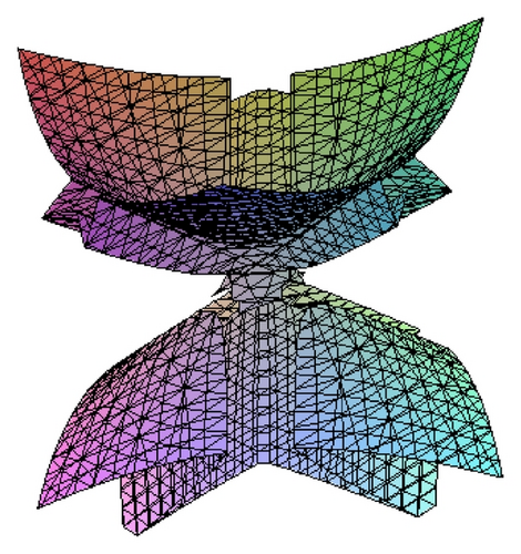
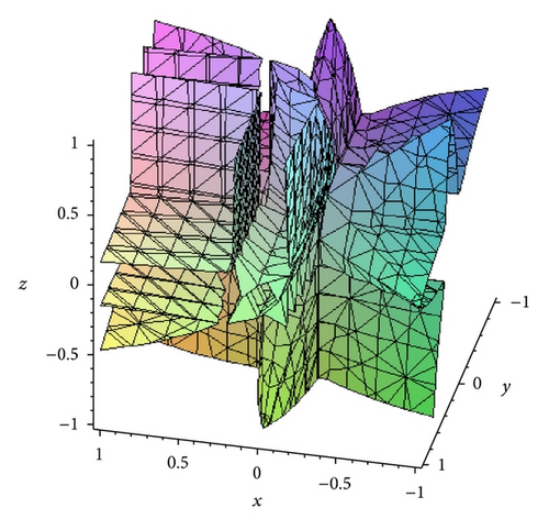
If p = 0, the boundaries of instability of solutions of (70) are constructed in the plane of parameters a1, a2, and a3 for different values ρ (see Figure 1 where some admissible boundaries are constructed).


Acknowledgment
The first author was supported by the Grant no P201/11/0768 of Czech Grant Agency (Prague).


