Volume 2013, Issue 1 127321
Research Article
Open Access

Extinction and Ergodic Property of Stochastic SIS Epidemic Model with Nonlinear Incidence Rate

Qixing Han

Qixing Han

School of Mathematics and Statistics, Northeast Normal University, Changchun 130024, China nenu.edu.cn

School of Mathematics, Changchun Normal University, Changchun 130032, China cncnc.edu.cn

Search for more papers by this author
Daqing Jiang

Corresponding Author

Daqing Jiang

School of Mathematics and Statistics, Northeast Normal University, Changchun 130024, China nenu.edu.cn

Search for more papers by this author
Chengjun Yuan

Chengjun Yuan

School of Mathematics and Computer, Harbin University, Harbin 150086, China hrbust.edu.cn

Search for more papers by this author
First published: 04 December 2013
Citations: 2
Academic Editor: Peixuan Weng

Abstract

We investigate a stochastic SIS model with nonlinear incidence rate. We show that there exists a unique nonnegative solution to the system, and condition for the infectious individuals I(t) to be extinct is given. Moreover, we prove that the system has ergodic property. Finally, computer simulations are carried out to verify our results.

1. Introduction

More attention has been paid to the epidemics models in order to monitor and curb the spread of some human diseases. A classical model is proposed by Kermack and McKendrick in 1927 [1]. They divided the population into three classes denoted by S(t), I(t), and R(t), which expressed the number of susceptible individuals, infective individuals, and removed individuals at time t, respectively. The model is called susceptible-infected-removed (SIR) model, and SIR models were investigated by many researchers [24].

However some diseases, such as some sexually transmitted and bacterial diseases, do not have permanent immunity. In [5], they introduced a SIS model to describe the spread of the disease, which takes the following form:
()
with initial values S0 + I0 = N. N is the total size of the population. Where S(t) and I(t) express the number of susceptible individuals and infective individuals at time t, respectively, μ is the per capita birth (and death) rate, γ is the rate at which infected individuals become cured, and β is the per capita contact rate. In model (1), they assumed that a rate of contacts by an infective individual with a susceptible individual is proportional to population size, and model (1) has been well studied [6].
In fact, population dynamics is inevitably affected by environmental white noise, which is always present. Since the parameters in the deterministic models are constant, they have some limitations when we describe the epidemics systems. Some researchers have paid their attention to the stochastic epidemics model [79]. Especially, in [10], Gray et al. consider that the parameter β in (1) is perturbed with
()
where B(t) is Brownian motions and σ represents the intensities of the white noise. Corresponding to the deterministic model system (1), the stochastic system takes the following form:
()
Since S(t) + I(t) = N, then (3) is reduced to
()
For model (4), they pointed out that
  • (i)

    if (βN/(μ + γ) − σ2N2/2(μ + γ)) < 1 and σ2β/N, the disease I(t) will die out with probability one;

  • (ii)

    if (βN/(μ + γ) − σ2N2/2(μ + γ)) > 1, then model (4) has a unique stationary distribution.

The incidence rate in (4) is bilinear, and several authors pointed out that the disease transmission process may have a nonlinear incidence rate [11, 12]. In [13], Xiao and Ruan propose an incidence rate
()
where α is the parameter that measures the psychological or inhibitory effect, and 1/(1 + αI2) describes the psychological or inhibitory effect from the behavioral change of the susceptible individuals when the number of infective individuals is very large. It can be used to explain some phenomena; for example, the outbreak of severe acute respiratory syndrome (SARS) had such psychological effects on the general public [14]: for a very large number of infective individuals, the infection force may decrease as the number of infective individuals increases. Some control measures and policies, such as border screening, mask wearing, quarantine, isolation, and so forth, can decrease the infection rate although the number of infective individuals was getting relatively larger. Equation (1) with nonlinear incidence rate (5) and the disturbed parameter β () can be written as follows:
()
The parameters appearing in (6) have the same meaning as those above. Given that S(t) + I(t) = N, it is sufficient to study the SDE for I(t),
()
with initial value I(0) = I0 ∈ (0, N). Notice that when α = 0, system (7) becomes (4). In this paper, we will analyze the dynamical behaviors of (7).

The organization of this paper is as follows. In the next section, we show that there exists a unique positive solution to (7). In Section 3, we carry out a qualitative analysis of the model (7) and extinction conditions for I(t) is derived. We prove that the system has ergodic property under some condition in Section 4. In Section 5, we present some numerical simulations to illustrate our mathematical findings. A brief conclusion is given in Section 6.

Throughout this paper, let (Ω, , P) be a complete probability space with a filtration {t} t≥0 satisfying the usual conditions (i.e., it is increasing and right continuous while 0 contains all P-null sets) and let B(t) be a scalar Brownian motion defined on the probability space.

2. Existence and Uniqueness of the Global Positive Solution

In order for the model to make sense, we need to show the solution is global and nonnegative. However, theorem of existence and uniqueness (cf. Arnold [15] and Mao [16]) is not satisfied in (7). By using tools established by Mao et al. [17], we will show existence and uniqueness of the global positive solution of (7).

Theorem 1. For any given initial data I(0) = I0 ∈ (0, N), there exists a unique solution I(t)∈(0, N) for all t ≥ 0 with probability 1.

Proof. It is obvious that the coefficients of the SDE (7) are locally continuous. For any given initial data I(0) = I0 ∈ (0, N), there exists a unique maximal local solution I(t) on t ∈ [0, τe), where τe is the explosion time. In order to show that the solution is global, it is sufficient to show τe = a.s. Let m0 > 0 be sufficiently large so that I0 lies within the interval [1/m0, N − 1/m0]. For each integer mm0, we define the stopping time

()
where, throughout this paper, we set inf   = (as usual denotes the empty set). It is clear that τm is increasing as m. Let τ = lim mτm, whence ττe. It is easy to show that τ = a.s. implies τe = a.s. and I(t)∈(0, N) a.s. for all t ≥ 0. Therefore, to complete this proof, it is enough to show that τ = a.s.

Define a function V : (0, N) → R+   as follows:

()
By Itô’s formula, we get
()
where
()
By almost the same method in the proof of [10], the desired result will be obtained.

3. Extinction

In this section, we will point out the condition for I(t) to be extinct. We firstly do some preparation work.

Consider the following stochastic equation:
()
and assume that the coefficients σ : JR, b : JR satisfy
  • (1)

    σ2(x) > 0, ∀xJ,

  • (2)

    xI, ∃ϵ > 0 such that ,

where J = (l, r); −l < r.

Lemma 2 (see [18].)Assume that (1) and (2) hold, and let X(t) be a weak solution of (12) in J, with nonrandom initial condition X0 = xJ. Let p be given by

()
If p(l+)>−, p(r−) = , then
()

Theorem 3. If , then for any initial data I(0) = I0 ∈ (0, N), the solution of SDE (7) has the following property:

()
that is, the disease dies out with probability one.

Proof. Applying Lemma 2 with b(x) = β(Nx)x/(1 + αx2)−(μ + γ)x, σ(x) = σ(Nx)x/(1 + αx2) and cJ = (0, N), we can compute

()
Clearly, conditions (1) and (2) are satisfied. By calculation, we have
()

We see that

()
Let 1/(Ns) = t; we obtain that
()
Clearly,
()
When , we have
()
that is,
()
It can be straightly shown by Lemma 2 that
()
The proof is therefore completed.

4. Ergodic Property

In this section, we show that the small perturbation forces the infective individuals to be ergodic.

Theorem 4. If , then, for any initial data I(0) = I0 ∈ (0, N), the solution of SDE (7) is ergodic.

Proof. If , we get

()
It follows from (20) that
()
Besides,
()
Let t = N/(Nx) − 1; then
()
When , that is, 2 − (2(βN − (μ + γ))/σ2N2) < 1, we have
()
The conditions of Theorem 1.16 in Kutoyants [19] follow from (24), (25), and (28). Therefore I(t) is ergodic, and the invariant density is given by
()
where C is a constant.

Remark 5. If α = 0, then

()
By the property of density function, we have
()
Let x = Nt/(t + 1); then
()
which implies
()
Next, we compute E(X):
()
This together with (33) shows that
()
Similarly, we have
()
Consequently,
()
When α = 0, model (7) becomes (4), and the mean and variance of the stationary distribution of model (4) are the same as the results in [10].

5. Simulations

We utilize the method developed in [20] to illustrate our findings. We have the corresponding discretization equation:
()
where εk are the Gaussian random variables N(0,1).

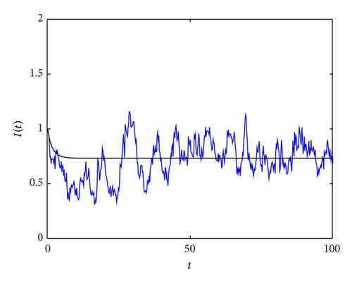
Using the discretized equation and with the help of Matlab software, choosing the appropriate parameters N = 2, β = 0.5, μ = 0.2, γ = 0.3, and α = 0.5, we get simulations of system (7) and the corresponding deterministic system.

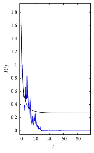
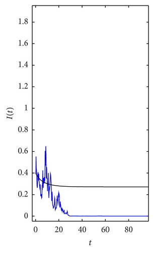
In Figure 1, we choose initial values I(0) = 1.8 and 0.4, respectively, σ = 0.6, noting that 2(βNμγ)/σ2N2 = 0.694 < 1, as the case in Theorem 3 expected, for any initial value I0 ∈ (0,2), the large white noise leads to the extinction of I(t) and the solution of system (7) tends to zero; that is, the disease dies out. While the solution of corresponding deterministic system does not tend to zero.
Details are in the caption following the image
The solution I(t) of SIS model (7) compared to the deterministic system with different initial value I(0) = 1.8 and 0.4, σ = 0.6. The blue line represents the solution of stochastic system, and the black line represents the solution of the corresponding deterministic system.

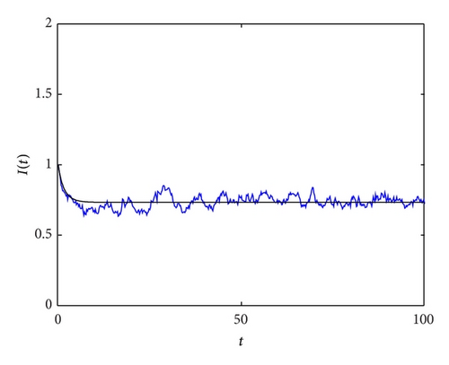
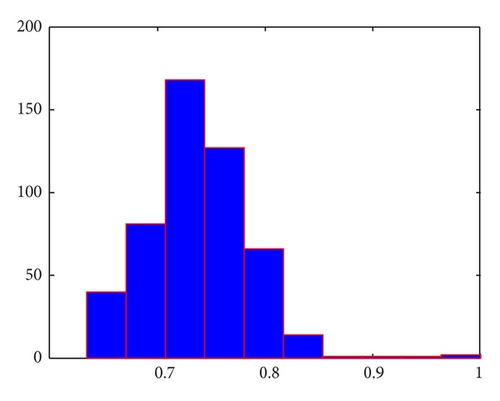
In Figure 2, we choose σ = 0.2 and 0.05, respectively, with initial values I(0) = 1.5, which satisfy the cases in Theorem 4; that is, 2(βNμγ)/σ2N2 > 1. From the left picture in Figure 2, we can see that the solution of system (7) is fluctuating in a small neighborhood, and there is a stationary distribution (see the histogram in Figures 2(b) and 2(d)); the disease becomes endemic.
Details are in the caption following the image
The solution I(t) of SIS model (7) and its histogram with differing value of σ = 0.2,0.05.
Details are in the caption following the image
The solution I(t) of SIS model (7) and its histogram with differing value of σ = 0.2,0.05.
Details are in the caption following the image
The solution I(t) of SIS model (7) and its histogram with differing value of σ = 0.2,0.05.
Details are in the caption following the image
The solution I(t) of SIS model (7) and its histogram with differing value of σ = 0.2,0.05.

6. Conclusion

In this paper, we analyze the dynamic behaviors of a stochastic SIS model with nonlinear incidence rate, under the assumption that the population lives in an environment subjected to random fluctuations which mainly affect the disease transmission term. First of all, we show that there exists a unique positive solution in system (7). Moreover, we obtain the threshold between prevalence and extinction of the disease; that is, if , the disease will die out with probability one; if , I(t) is ergodic, which means the disease will become endemic. Finally, we illustrate our results with computer simulations.

We see that if α = 0, (7) becomes (4), which is studied in [10]; they show that if βN/(μ + γ) − σ2N2/2(μ + γ) < 1 and σ2β/N, the disease I(t) will die out with probability one. Obviously, βN/(μ + γ) − σ2N2/2(μ + γ) < 1 and are equivalent. The condition σ2β/N, however, is not necessary in our investigation. In addition, if , the invariant density is obtained, which is not mentioned in [10].

An extension of our work is to consider a stochastic SIS model with the general incidence rate βIpS/(1 + αIq), and it is currently a work in progress.

Acknowledgments

The work was supported by the Program for Changjiang Scholars and Innovative Research Team in University, NSF of China (nos. 11371085 and 11101072); the Ph.D. Programs Foundation of Ministry of China (no. 200918); and the Nature Science Foundation of Changchun Normal University (no. 2010007).

      The full text of this article hosted at iucr.org is unavailable due to technical difficulties.