An efficient iterative algorithm is presented to solve a system of linear matrix equations A₁X₁B₁ + A₂X₂B₂ = E, C₁X₁D₁ + C₂X₂D₂ = F with real matrices X₁ and X₂. By this iterative algorithm, the solvability of the system can be determined automatically. When the system is consistent, for any initial matrices and , a solution can be obtained in the absence of roundoff errors, and the least norm solution can be obtained by choosing a special kind of initial matrix. In addition, the unique optimal approximation solutions and to the given matrices and in Frobenius norm can be obtained by finding the least norm solution of a new pair of matrix equations , where , . The given numerical example demonstrates that the iterative algorithm is efficient. Especially, when the numbers of the parameter matrices A₁, A₂, B₁, B₂, C₁, C₂, D₁, D₂ are large, our algorithm is efficient as well.

1. Introduction

Throughout the paper, we denote the set of all m × n real matrix by R^m×n, the transpose matrix of A by A^T, the identity matrix of order n by I_n, the Kronecker product of A and B by A ⊗ B, the mn × 1 vector formed by the vertical concatenation of the respective columns of a matrix A ∈ R^m×n by vec (A), the trace of a matrix A by tr (A), and the Frobenius norm of a matrix A by ∥A∥ where .

In this paper, we consider the following two problems.

Problem 1. For the given matrices A₁ ∈ R^p×k, A₂ ∈ R^p×m, B₁ ∈ R^r×q, B₂ ∈ R^n×q, C₁ ∈ R^s×k, C₂ ∈ R^s×m, D₁ ∈ R^r×t, D₂ ∈ R^n×t, E ∈ R^p×q, and F ∈ R^s×t, find X₁ ∈ R^k×r and X₂ ∈ R^m×n such that

()

Problem 2. When Problem 1 is consistent, let S denote the solution set of the pair of matrix equation (1). For the given matrices , , find such that

()

Problem 2 is to find the optimal approximation solutions to the given matrices in the solution set of Problem 1. It occurs frequently in experiment design (see, for instance, [1]). In the recent years, the matrix optimal approximation problem has been studied extensively (e.g., [2–13]).

The research on solving matrix equation pair has been actively ongoing for the last 30 years or more. For instance, Mitra [14] gave conditions for the existence of a solution and a representation of the general common solution to AXB = E, CXD = F. Shinozaki and Sibuya [15] and van der Woude [16] discussed conditions for the existence of a common solution to AXB = E, CXD = F. Navarra et al. [5] derived sufficient and necessary conditions for the existence of a common solution to AXB = E, CXD = F. Yuan [13] obtained an analytical expression of the least-squares solutions of AXB = E, CXD = F by using the generalized singular value decomposition (GSVD) of matrices. Dehghan and Hajarian [17] presented some examples to show a motivation for studying the general coupled matrix equations , i = 1,2, …, l, and [18] constructed an iterative algorithm to solve the general coupled matrix equations , i = 1,2, …, p. Wang [19, 20] gave the centrosymmetric solution to the system of quaternion matrix equations A₁X = C₁, A₃XB₃ = C₃. Wang [21] also solved a system of matrix equations over arbitrary regular rings with identity.

Recently, some finite iterative algorithms have also been developed to solve matrix equations. Ding et al. [22, 23] and Xie et al. [24, 25] studied the iterative solutions of matrix equations AXB = F and A_iXB_i = F_i and generalized Sylvester matrix equations AXB + CXD = F and AXB + CX^TD = F. They presented a gradient based and a least-squares based iterative algorithms for the solution. Li et al. [26, 27] and Zhou et al. [28, 29] considered iterative method for some coupled linear matrix equations. Deng et al. [30] studied the consistent conditions and the general expressions about the Hermitian solutions of the matrix equations (AX, XB) = (C, D) and designed an iterative method for its Hermitian minimum norm solutions. Li and Wu [31] gave symmetric and skew-antisymmetric solutions to certain matrix equations A₁X = C₁, XB₃ = C₃ over the real quaternion algebra H. For more studies on iterative algorithms on coupled matrix equations, we refer to [3, 10–12, 17, 32–37]. Peng et al. [6] presented iterative methods to obtain the symmetric solutions of AXB = E, CXD = F. Sheng and Chen [8] presented a finite iterative method; when AXB = E, CXD = F is consistent. Liao and Lei [38] presented an analytical expression of the least-squares solution and an algorithm for AXB = E, CXD = F with the minimum norm. Peng et al. [7] presented an algorithm for the least-squares reflexive solution. Dehghan and Hajarian [2] presented an iterative algorithm for solving a pair of matrix equations AXB = E, CXD = F over generalized centrosymmetric matrices. Cai and Chen [39] presented an iterative algorithm for the least-squares bisymmetric solutions of the matrix equations AXB = E, CXD = F. Yin and Huang [40] presented an iterative algorithm to solve the least squares generalized reflexive solutions of the matrix equations AXB = E, CXD = F.

However, to our knowledge, there has been little information on finding the solutions to the system (1) by iterative algorithm. In this paper, an efficient iterative algorithm is presented to solve the system (1) for any real matrices X₁, X₂. The suggested iterative algorithm, automatically determines the solvability of equations pair (1). When the pair of equations is consistent, then, for any initial matrices and , the solution can be obtained in the absence of round errors, and the least norm solution can be obtained by choosing a special kind of initial matrix. In addition, the unique optimal approximation solutions and to the given matrices and in Frobenius norm can be obtained by finding the least norm solution of a new pair of matrix equations , , where , . The given numerical examples demonstrate that our iterative algorithm is efficient. Especially, when the numbers of the parameter matrices A₁, A₂, B₁, B₂, C₁, C₂, D₁, D₂ are large, our algorithm is efficient as well while the algorithm of [32] is not convergent. That is, our algorithm has merits of good numerical stability and ease to program.

The rest of this paper is outlined as follows. In Section 2, we first propose an efficient iterative algorithm for solving Problem 1; then we give some properties of this iterative algorithm. We show that the algorithm can obtain a solution group (the least Frobenius norm solution group) for any (special) initial matrix group in the absence of roundoff errors. In Section 3, a numerical example is given to illustrate that our algorithm is quite efficient.

2. Iterative Algorithm for Solving Problems 1 and 2

In this section, we present the iterative algorithm for the consistence of the system (1).

Algorithm 3. (1) Input matrices A₁ ∈ R^p×k, A₂ ∈ R^p×m, B₁ ∈ R^r×q, B₂ ∈ R^n×q, C₁ ∈ R^s×k, C₂ ∈ R^s×m, D₁ ∈ R^r×t, D₂ ∈ R^n×t, E ∈ R^p×q, F ∈ R^s×t, , and (where , are any initial matrices).

(2) Calculate

()

(3) If (k = 1,2, …), then stop. Otherwise,

()

(4) Calculate

()

Go to (3).

Lemma 4. In Algorithm 3, the choice of β^k makes ∥diag (E^k+1, F^k+1)∥ reach a minimum and diag (E^k+1, F^k+1) and orthogonal to each other.

Proof. From Algorithm 3, we have

()

From the above, the condition of ∥diag (E^k+1, F^k+1)∥ reaching a minimum is

()

On the other hand, if the choice of β^k makes diag (E^k+1, F^k+1) and orthogonal to each other, that is, , we can have the same β^k as (7).

Theorem 5. Algorithm 3 is bound to be convergent.

Proof. From Algorithm 3 and Lemma 4 we have

()

such that

()

From (9), we know that Algorithm 3 is convergent.

Lemma 6 (see [41].)Suppose that the consistent system of linear equations My = b has a solution y₀ ∈ R(M^T); then y₀ is the least Frobenius norm solution of the system of linear equations.

Theorem 7. Assume that the system (1) is consistent. Let , be initial matrices where Y ∈ R^p×q, Z ∈ R^s×t are any initial matrices, or, especially, , ; then the solution generated by Algorithm 3 is the least Frobenius norm solution to (1).

Proof. If (1) is consistent, from , , using Algorithm 3, we have the iterative solution pair of (1) as the following:

()

We know that (1) is equivalent to the system

()

From (10) and (11) we have

()

where R(*) is the column space of matrix *.

Considering Lemma 6, with the initial matrices , , where Y ∈ R^p×q, Z ∈ R^s×t are arbitrary, or, especially, and , then the solution pair generated by Algorithm 3 is the least Frobenius norm solution of the matrix equations (1).

Suppose that Problem 1 is consistent. Obviously the solution set S of (1) is nonempty. For given matrices pair

, we can write

()

Let

, and

. Then Problem 2 is equivalent to find the least Frobenius norm solution pair of the system

()

which can be obtained using Algorithm 3 with the initial matrix pair

where Y ∈ R^p×q and Z ∈ R^s×t are arbitrary, or especially,

, and the solution of the matrix optimal approximation Problem 2 can be represented as

3. An Example

In this section, we show a numerical example to illustrate the efficiency of Algorithm 3. All computations are performed by MATLAB 7. For the influence of the error of calculation, we consider the matrix R as a zero matrix if ∥R∥ < 10⁻¹⁰.

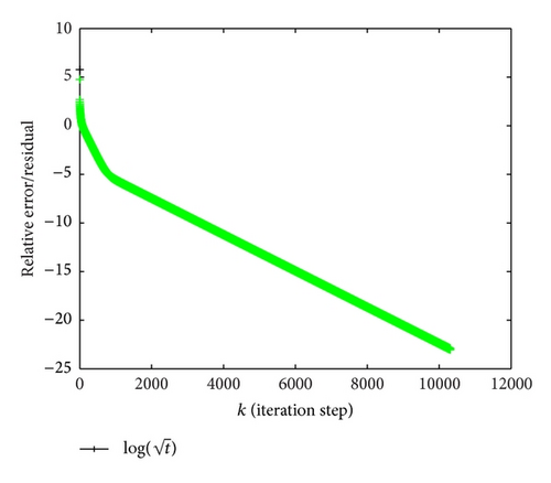
Example 1. Consider the solution of the linear matrix equations

()

where

()

In this example, the numbers of the parameter matrices A₁, A₂, B₁, B₂, C₁, C₂, D₁, D₂ are larger than the numbers of the parameter matrices in the example of [32]. It can be verified that these matrix equations are consistent and have the solution as

()

Let

()

(1) Using Algorithm 3 and iterate 10309 steps, we obtain the least Frobenius norm solution pair of the matrix equation in Example 1 as follows:

()

The obtained sequence ∥ΔX∥ are presented in Figure 1.

Details are in the caption following the image — **Figure 1**
Open in figure viewer PowerPoint

The obtained sequence ∥ΔX∥ by Algorithm 3 for Example 1.

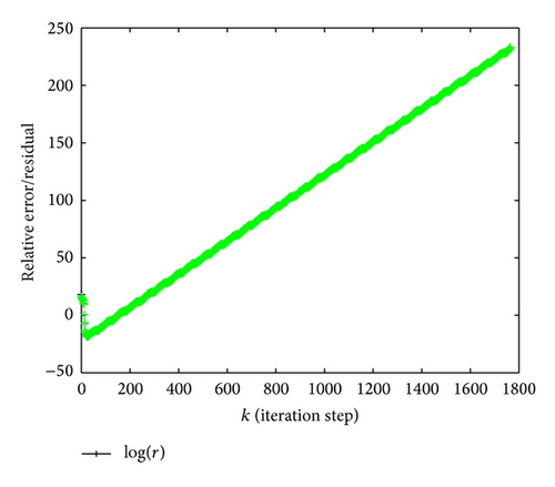
(2) Using the algorithm of [32], to this example, the iteration is not convergent. The obtained result is presented in Figure 2.

This numerical example demonstrates that our algorithm has merits of good numerical stability and ease to program.

Acknowledgments

This research was supported by the Grants from the Key Project of Scientific Research Innovation Foundation of Shanghai Municipal Education Commission (13ZZ080), the National Natural Science Foundation of China (11171205), the Natural Science Foundation of Shanghai (11ZR1412500), and the Nature Science Foundation of Anhui Provincial Education (ky2008b253, KJ2013A248).

References

1 Meng T., C. Leondes, Experimental design and decision support, in expert systems, The Technology of Knowledge Management and Decision Making for the 21st Century, 2001, 1, Academic Press, New York, NY, USA.
Google Scholar
2 Dehghan M. and Hajarian M., An iterative algorithm for solving a pair of matrix equations AYB = E, CYD = F over generalized centro-symmetric matrices, Computers & Mathematics with Applications. (2008) 56, no. 12, 3246–3260, https://doi.org/10.1016/j.camwa.2008.07.031, MR2474579.
10.1016/j.camwa.2008.07.031
Web of Science® Google Scholar
3 Dehghan M. and Hajarian M., An iterative algorithm for the reflexive solutions of the generalized coupled Sylvester matrix equations and its optimal approximation, Applied Mathematics and Computation. (2008) 202, no. 2, 571–588, https://doi.org/10.1016/j.amc.2008.02.035, MR2435692, ZBL1154.65023.
10.1016/j.amc.2008.02.035
Web of Science® Google Scholar
4 Andrew A. L., Solution of equations involving centrosymmetric matrices, Technometrics. (1973) 15, no. 2, 405–407.
10.1080/00401706.1973.10489052
Web of Science® Google Scholar
5 Navarra A., Odell P. L., and Young D. M., A representation of the general common solution to the matrix equations A₁XB₁ = C₁ and A₂XB₂ = C₂ with applications, Computers & Mathematics with Applications. (2001) 41, no. 7-8, 929–935, https://doi.org/10.1016/S0898-1221(00)00330-8, MR1826896, ZBL0983.15016.
10.1016/S0898-1221(00)00330-8
Web of Science® Google Scholar
6 Peng Y.-X., Hu X.-Y., and Zhang L., An iterative method for symmetric solutions and optimal approximation solution of the system of matrix equations A₁XB₁ = C₁, A₂XB₂ = C₂, Applied Mathematics and Computation. (2006) 183, no. 2, 1127–1137, https://doi.org/10.1016/j.amc.2006.05.124, MR2294070, ZBL1134.65032.
10.1016/j.amc.2006.05.124
Web of Science® Google Scholar
7 Peng Z.-H., Hu X.-Y., and Zhang L., An efficient algorithm for the least-squares reflexive solution of the matrix equation A₁XB₁ = C₁; A₂XB₂ = C₂, Applied Mathematics and Computation. (2006) 181, no. 2, 988–999, https://doi.org/10.1016/j.amc.2006.01.071, MR2269978, ZBL1115.65048.
10.1016/j.amc.2006.01.071
Web of Science® Google Scholar
8 Sheng X. and Chen G., A finite iterative method for solving a pair of linear matrix equations (AXB, CXD) = (E, F), Applied Mathematics and Computation. (2007) 189, no. 2, 1350–1358, https://doi.org/10.1016/j.amc.2006.12.026, MR2331808, ZBL1133.65026.
10.1016/j.amc.2006.12.026
Web of Science® Google Scholar
9 Li N. and Wang Q. W., Iterative algorithm for solving a class of quaternion matrix equation over the generalized (P, Q)-reflexive matrices, Abstract and Applied Analysis. (2013) 2013, 15, 831656, https://doi.org/10.1155/2013/831656.
10.1155/2013/831656
Google Scholar
10 Wu A.-G., Feng G., Duan G.-R., and Wu W.-J., Finite iterative solutions to a class of complex matrix equations with conjugate and transpose of the unknowns, Mathematical and Computer Modelling. (2010) 52, no. 9-10, 1463–1478, https://doi.org/10.1016/j.mcm.2010.06.010, MR2719531, ZBL1205.15027.
10.1016/j.mcm.2010.06.010
Web of Science® Google Scholar
11 Wu A.-G., Feng G., Duan G.-R., and Wu W.-J., Iterative solutions to coupled Sylvester-conjugate matrix equations, Computers & Mathematics with Applications. (2010) 60, no. 1, 54–66, https://doi.org/10.1016/j.camwa.2010.04.029, MR2651883, ZBL1198.65083.
10.1016/j.camwa.2010.04.029
Web of Science® Google Scholar
12 Wu A.-G., Li B., Zhang Y., and Duan G.-R., Finite iterative solutions to coupled Sylvester-conjugate matrix equations, Applied Mathematical Modelling. (2011) 35, no. 3, 1065–1080, https://doi.org/10.1016/j.apm.2010.07.053, MR2740850, ZBL1211.15024.
10.1016/j.apm.2010.07.053
Web of Science® Google Scholar
13 Yuan Y.-X., On the minimum norm solution of matrix equation AXB = E; CXD = F, Journal of East China Shipbuilding Institute. (2001) 15, no. 3, 34–37, 2-s2.0-0035361105.
Google Scholar
14 Mitra S. K., Common solutions to a pair of linear matrix equations A₁XB₁ = C₁ and A₂XB₂ = C₂, 1973, 74, 213–216, MR0320028, ZBL0262.15010.
Google Scholar
15 Shinozaki N. and Sibuya M., Consistency of a pair of matrix equations with an application, Keio Science and Technology Reports. (1975) 27, no. 10, 141–146, MR0382306.
Google Scholar
16 van der Woude J. W., Freeback decoupling and stabilization for linear systems with multiple exogenous variables [Ph.D. thesis], 1987, Technical University of Eindhoven, Eindhoven, The Netherlands.
Google Scholar
17 Dehghan M. and Hajarian M., The general coupled matrix equations over generalized bisymmetric matrices, Linear Algebra and Its Applications. (2010) 432, no. 6, 1531–1552, https://doi.org/10.1016/j.laa.2009.11.014, MR2580446, ZBL1187.65042.
10.1016/j.laa.2009.11.014
Web of Science® Google Scholar
18 Dehghan M. and Hajarian M., The reflexive and anti-reflexive solutions of a linear matrix equation and systems of matrix equations, The Rocky Mountain Journal of Mathematics. (2010) 40, no. 3, 825–848, https://doi.org/10.1216/RMJ-2010-40-3-825, MR2665204, ZBL1198.15011.
10.1216/RMJ-2010-40-3-825
Web of Science® Google Scholar
19 Wang Q.-W., Sun J.-H., and Li S.-Z., Consistency for bi(skew)symmetric solutions to systems of generalized Sylvester equations over a finite central algebra, Linear Algebra and Its Applications. (2002) 353, 169–182, https://doi.org/10.1016/S0024-3795(02)00303-8, MR1919635, ZBL1004.15017.
10.1016/S0024-3795(02)00303-8
Web of Science® Google Scholar
20 Wang Q.-W., Bisymmetric and centrosymmetric solutions to systems of real quaternion matrix equations, Computers & Mathematics with Applications. (2005) 49, no. 5-6, 641–650, https://doi.org/10.1016/j.camwa.2005.01.014, MR2134960, ZBL1138.15003.
10.1016/j.camwa.2005.01.014
Web of Science® Google Scholar
21 Wang Q.-W., A system of matrix equations and a linear matrix equation over arbitrary regular rings with identity, Linear Algebra and Its Applications. (2004) 384, 43–54, https://doi.org/10.1016/j.laa.2003.12.039, MR2055342, ZBL1058.15015.
10.1016/j.laa.2003.12.039
Web of Science® Google Scholar
22 Ding F., Liu P. X., and Ding J., Iterative solutions of the generalized Sylvester matrix equations by using the hierarchical identification principle, Applied Mathematics and Computation. (2008) 197, no. 1, 41–50, https://doi.org/10.1016/j.amc.2007.07.040, MR2396289, ZBL1143.65035.
10.1016/j.amc.2007.07.040
Web of Science® Google Scholar
23 Ding J., Liu Y., and Ding F., Iterative solutions to matrix equations of the form A_iXB_i = F_i, Computers & Mathematics with Applications. (2010) 59, no. 11, 3500–3507, https://doi.org/10.1016/j.camwa.2010.03.041, MR2646321, ZBL1197.15009.
10.1016/j.camwa.2010.03.041
Web of Science® Google Scholar
24 Xie L., Ding J., and Ding F., Gradient based iterative solutions for general linear matrix equations, Computers & Mathematics with Applications. (2009) 58, no. 7, 1441–1448, https://doi.org/10.1016/j.camwa.2009.06.047, MR2555281, ZBL1189.65083.
10.1016/j.camwa.2009.06.047
Web of Science® Google Scholar
25 Xie L., Liu Y., and Yang H., Gradient based and least squares based iterative algorithms for matrix equations AXB + CX^TD = F, Applied Mathematics and Computation. (2010) 217, no. 5, 2191–2199, https://doi.org/10.1016/j.amc.2010.07.019, MR2727965, ZBL1210.65097.
10.1016/j.amc.2010.07.019
Web of Science® Google Scholar
26 Li Z.-Y., Wang Y., Zhou B., and Duan G.-R., Least squares solution with the minimum-norm to general matrix equations via iteration, Applied Mathematics and Computation. (2010) 215, no. 10, 3547–3562, https://doi.org/10.1016/j.amc.2009.10.052, MR2578938, ZBL1186.65047.
10.1016/j.amc.2009.10.052
Web of Science® Google Scholar
27 Li Z.-Y., Zhou B., Wang Y., and Duan G.-R., Numerical solution to linear matrix equation by finite steps iteration, IET Control Theory & Applications. (2010) 4, no. 7, 1245–1253, https://doi.org/10.1049/iet-cta.2009.0015, MR2768248.
10.1049/iet-cta.2009.0015
Web of Science® Google Scholar
28 Zhou B., Lam J., and Duan G.-R., On Smith-type iterative algorithms for the Stein matrix equation, Applied Mathematics Letters. (2009) 22, no. 7, 1038–1044, https://doi.org/10.1016/j.aml.2009.01.012, MR2522996, ZBL1179.15016.
10.1016/j.aml.2009.01.012
Web of Science® Google Scholar
29 Zhou B., Lam J., and Duan G.-R., Gradient-based maximal convergence rate iterative method for solving linear matrix equations, International Journal of Computer Mathematics. (2010) 87, no. 1–3, 515–527, https://doi.org/10.1080/00207160802123458, MR2598758, ZBL1188.65058.
10.1080/00207160802123458
Web of Science® Google Scholar
30 Deng Y.-B., Bai Z.-Z., and Gao Y.-H., Iterative orthogonal direction methods for Hermitian minimum norm solutions of two consistent matrix equations, Numerical Linear Algebra with Applications. (2006) 13, no. 10, 801–823, https://doi.org/10.1002/nla.496, MR2278194, ZBL1174.65382.
10.1002/nla.496
Web of Science® Google Scholar
31 Li Y.-T. and Wu W.-J., Symmetric and skew-antisymmetric solutions to systems of real quaternion matrix equations, Computers & Mathematics with Applications. (2008) 55, no. 6, 1142–1147, https://doi.org/10.1016/j.camwa.2007.06.015, MR2394352, ZBL1143.15012.
10.1016/j.camwa.2007.06.015
Web of Science® Google Scholar
32 Dehghan M. and Hajarian M., An efficient algorithm for solving general coupled matrix equations and its application, Mathematical and Computer Modelling. (2010) 51, no. 9-10, 1118–1134, https://doi.org/10.1016/j.mcm.2009.12.022, MR2608897, ZBL1208.65054.
10.1016/j.mcm.2009.12.022
Google Scholar
33 Dehghan M. and Hajarian M., On the reflexive and anti-reflexive solutions of the generalised coupled Sylvester matrix equations, International Journal of Systems Science. (2010) 41, no. 6, 607–625, https://doi.org/10.1080/00207720903072357, MR2662731, ZBL1196.65081.
10.1080/00207720903072357
Web of Science® Google Scholar
34 Zhou B., Li Z.-Y., Duan G.-R., and Wang Y., Weighted least squares solutions to general coupled Sylvester matrix equations, Journal of Computational and Applied Mathematics. (2009) 224, no. 2, 759–776, https://doi.org/10.1016/j.cam.2008.06.014, MR2492909, ZBL1161.65034.
10.1016/j.cam.2008.06.014
Web of Science® Google Scholar
35 Jonsson I. and Kågström B., Recursive blocked algorithm for solving triangular systems. I. One-sided and coupled Sylvester-type matrix equations, ACM Transactions on Mathematical Software. (2002) 28, no. 4, 392–415, https://doi.org/10.1145/592843.592845, MR2003127.
10.1145/592843.592845
Web of Science® Google Scholar
36 Zhou B., Duan G.-R., and Li Z.-Y., Gradient based iterative algorithm for solving coupled matrix equations, Systems & Control Letters. (2009) 58, no. 5, 327–333, https://doi.org/10.1016/j.sysconle.2008.12.004, MR2512486, ZBL1159.93323.
10.1016/j.sysconle.2008.12.004
Web of Science® Google Scholar
37 Jonsson I. and Kågström B., Recursive blocked algorithm for solving triangular systems. II. Two-sided and generalized Sylvester and Lyapunov matrix equations, ACM Transactions on Mathematical Software. (2002) 28, no. 4, 416–435, https://doi.org/10.1145/592843.592846, MR2003128.
10.1145/592843.592846
Web of Science® Google Scholar
38 Liao A.-P. and Lei Y., Least-squares solution with the minimum-norm for the matrix equation (AXB, GXH) = (C, D), Computers & Mathematics with Applications. (2005) 50, no. 3-4, 539–549, https://doi.org/10.1016/j.camwa.2005.02.011, MR2165440, ZBL1087.65040.
10.1016/j.camwa.2005.02.011
Web of Science® Google Scholar
39 Cai J. and Chen G., An iterative algorithm for the least squares bisymmetric solutions of the matrix equations A₁XB₁ = C₁, A₂XB₂ = C₂, Mathematical and Computer Modelling. (2009) 50, no. 7-8, 1237–1244, https://doi.org/10.1016/j.mcm.2009.07.004, MR2568114, ZBL1190.65061.
10.1016/j.mcm.2009.07.004
Google Scholar
40 Yin F. and Huang G.-X., An iterative algorithm for the least squares generalized reflexive solutions of the matrix equations AXB = E; CXD = F, Abstract and Applied Analysis. (2012) 2012, 18, https://doi.org/10.1155/2012/857284, 857284, MR2898044, ZBL1242.65085.
10.1155/2012/857284
Google Scholar
41 Peng Y.-X., Hu X.-Y., and Zhang L., An iteration method for the symmetric solutions and the optimal approximation solution of the matrix equation AXB = C, Applied Mathematics and Computation. (2005) 160, no. 3, 763–777, https://doi.org/10.1016/j.amc.2003.11.030, MR2113117, ZBL1068.65056.
10.1016/j.amc.2003.11.030
Web of Science® Google Scholar

Citing Literature

All articles

Iterative Solution to a System of Matrix Equations

Abstract

1. Introduction

2. Iterative Algorithm for Solving Problems 1 and 2

3. An Example

Acknowledgments

References

Citing Literature

Figures

References

Information

About Wiley Online Library

Help & Support

Opportunities

Connect with Wiley

Iterative Solution to a System of Matrix Equations

Abstract

1. Introduction

2. Iterative Algorithm for Solving Problems 1 and 2

3. An Example

Acknowledgments

References

Citing Literature

Figures

References

Related

Information