This paper deals with an inverse problem for identifying an unknown source which depends only on one variable in two-dimensional Poisson equation, with the aid of an extra measurement at an internal point. Since this problem is illposed, we obtain the regularization solution by the modified regularization method. Furthermore, we obtain the Hölder-type error estimate between the regularization solution and the exact solution. The numerical results show that the proposed method is stable and the unknown source is recovered very well.

1. Introduction

Inverse source problem is an ill posed problem that has received considerable attention from many researches in a variety of fields, such as heat conduction, crack identification, electromagnetic theory, geophysical prospecting, and pollutant detection. For the heat source identification, there have been a large number of research results for different forms of heat source [1–8]. To the authors’ knowledge, there were also a lot of researches on identification of the unknown source in the Poisson equation adopted numerical algorithms, such as the logarithmic potential method [9], the projective method [10], the Green’s function method [11], the dual reciprocity boundary element method [12], the dual reciprocity method [13, 14], and the method of fundamental solution (MFS) [15]. But, by the regularization method, there are a few papers with strict theoretical analysis on identifying the unknown source.

In this paper, we consider the following inverse problem: to find a pair of functions (u(x, y), f(x)) which satisfy the Poisson equation on half unbounded domain as follows:

()

where f(x) is the unknown source depending only on one spatial variable and u(x, 1) = g(x) is the supplementary condition. In applications, input data g(x) can only be measured, and there will be measured data function g_δ(x) which is merely in L²(ℝ) and satisfies

()

where the constant δ > 0 represents a noise level of input data.

The problem (1.1) is mildly ill posed, and the degree of the ill posedness is equivalent to the second-order numerical differentiation. It is impossible to solve the problem (1.1) using classical methods. The major object of this paper is to use the modified regularization method to obtain the regularization solution. Meanwhile, the Hölder-type stability estimate between the regularization solution and the exact solution is obtained. In [16], the authors ever identified the unknown source on the Poisson equation on half band domain using separation of variables. But in this paper, we identified the unknown source on the Poisson equation on half unbounded domain using the Fourier Transform.

This paper is organized as follows. Section 2 analyzes the ill posedness of the identification of the unknown source and gives some auxiliary results. Section 3 gives a regularization solution and error estimate. Section 4 gives several numerical examples including both nonsmooth and discontinuous cases for the problem (1.1). Section 5 ends this paper with a brief conclusion.

2. Some Auxiliary Results

The ill posedness can be seen by solving the problem (1.1) in the Fourier domain. Let

denote the Fourier transform of f(x) ∈ L²(ℝ) which is defined by

()

The problem (2.2) can now be formulated in frequency space as follows:

()

The solution of the problem (2.2) is given by

()

So,

()

The unbounded function ξ²/(1 − e^−ξ) in (2.3) or (2.4) can be seen as an amplification factor of

when ξ → ∞. Therefore, when we consider our problem in L²(ℝ), the exact data function

must decay. But, in the applications, the input data g(x) can only be measured and can never be exact. Thus, if we try to obtain the unknown source f(x), high-frequency components in the error are magnified and can destroy the solution. In general, for an ill posed problem, the convergence rates of the regularization solution can only be given under prior assumptions on the exact solution; we impose an a priori bound on the exact solution f(x) as follows:

()

where E > 0 is a constant and

denotes the norm in the Sobolev space H^p(ℝ) defined by

()

Now we give some important lemmas as follows.

Lemma 2.1. If x > 1, the following inequality:

()

holds.

Lemma 2.2. As 0 < μ < 1, one obtains the following inequalities:

()

Proof. Let

()

The proof of the first inequality of (2.8) can be divided into three cases.

Case 1 (|ξ| ≥ ξ0 : = 1/μ). We obtain

()

Case 2 (1 < |ξ| < ξ0). We get

()

If 0 < p ≤ 2, the above inequality becomes

()

If p > 2, we get

()

Case 3 (|ξ| ≤ 1). We obtain

()

Combining (2.10) with (2.12), (2.13), and (2.14), we obtain the first inequality equation.

Let

()

The proof of the second inequality of (2.8) can also be divided into two cases.

Case 1 (|ξ| ≤ ξ0 : = 1/μ). We obtain

()

So,

()

Case 2 (|ξ| > ξ0). We obtain

()

Combining (2.17) with (2.18), (2.8) holds.

3. A Modified Regularization Method and Error Estimate

We modify (1.1), where a two-order derivation of f(x), is added, that is,

()

This is based on the modified regularization method which we learned from Eldén [17] who considered a standard inverse heat conduction problem and the idea initially came from Weber [18]. This method has been studied for solving various types of inverse problems [19–24]. We obtain a stable approximate solution of problem (1.1), that is,

()

where the parameter μ is regarded as a regularization parameter. The problem (3.2) can be formulated in frequency space as follows:

()

The solution to this problem is given by

()

Note that, for small μ, ξ²/(1 + ξ²μ²) is close to ξ². On the contrary, if |ξ| becomes large, |ξ²/(1 + ξ²μ²) | is bounded. So, f_δ,μ(x) is considered as an approximation of f(x).

Now we will give an error estimate between the regularization solution and the exact solution by the following theorem.

Theorem 3.1. Suppose f(x) is an exact solution of (1.1) given by (2.4) and f_δ,μ(x) is the regularized approximation to f(x) given by (3.5). Let g_δ(x) be the measured data at y = 1 satisfying (1.2). Moreover, one assumes the a priori bound (2.5) holds. If one selects

()

then one obtains the following error estimate:

()

Proof. From the Parseval formula and (2.3), (3.4), (2.6), (2.7), (2.8), (1.2), (2.5), and (3.6), we obtain

()

Remark 3.2. If 0 < p ≤ 2,

()

If p > 2,

()

Hence, f_δ,μ(x) can be regarded as the approximation of the exact solution f(x).

Remark 3.3. In general, the a priori bound E in (2.5) is unknown exactly in practice. But, if we choose μ = δ^1/(p+2), we can also obtain

()

This choice is useful in concrete computation.

4. Several Numerical Examples

In this section, we present three numerical examples intended to illustrate the usefulness of the proposed method. The numerical results are presented, which verify the validity of the theoretical results of this method.

The numerical examples were constructed in the following way. First we selected the exact solution f(x) of problem (1.1) and obtained the exact data function g(x) using (2.3) or (2.4). Then, we added a normally distributed perturbation to each data function giving vectors g_δ. Finally, we obtained the regularization solutions using (3.4) or (3.5).

In the following, we first give an example which has the exact expression of the solutions (u(x, y), f(x)).

Example 4.1. It is easy to see that the function

()

and the function

()

are satisfied with the problem (1.1) with exact data

()

Suppose that the sequence

represents samples from the function g(x) on an equidistant grid and n is even. Then we add a random uniformly perturbation to each data, which forms the vector g_δ, that is,

()

where

()

The function “randn(·)” generates arrays of random numbers whose elements are normally distributed with mean 0, variance σ² = 1. “Randn(size(g))” returns an array of random entries that is of the same size as g. The total noise level δ can be measured in the sense of root mean square error (RMSE) according to

()

Moreover, we need to make the vector g_δ periodical [25], and then we take the discrete Fourier transform for the vector g_δ. The approximation of the regularization solution is computed by using FFT algorithm [25], and the range of variable x in the numerical experiment is [−10,10].

Example 4.2. Consider a piecewise smooth source:

()

Example 4.3. Consider the following discontinuous case:

()

From Figures 1–3, we can see that the smaller the ε, the better the computed approximation f_δ,μ(x).

Details are in the caption following the image — **Figure 1 (a)**
Open in figure viewer PowerPoint

Comparison between the exact solution and its computed approximations with various levels of noise for Example 4.1: (a) p = 1, (b) p = 2.

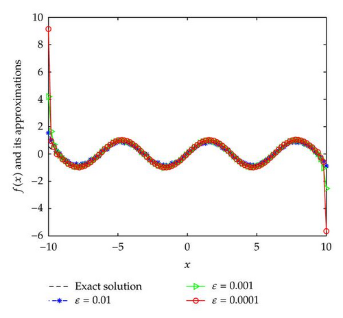
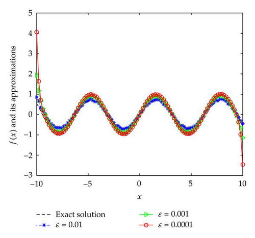
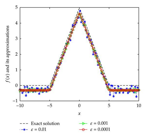
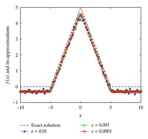
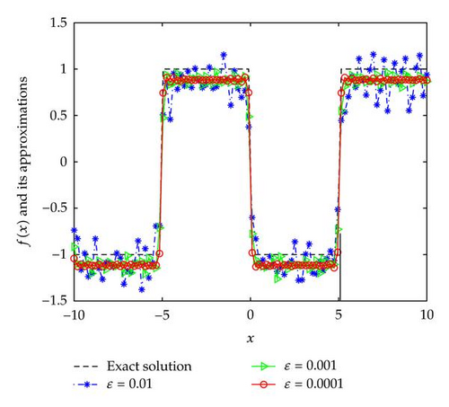
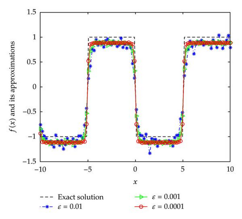
In Examples 4.2 and 4.3, since the direct problem with the source f(x) does not have an analytical solution, the data g(x) is obtained by solving the direct problem. From Figures 2 and 3, we can see that the numerical solutions are less ideal than that of Example 4.1. It is not difficult to see that the well-known Gibbs phenomenon and the recovered data near the nonsmooth and discontinuities points are not accurate. Taking into consideration the ill posedness of the problem, the results presented in Figures 2 and 3 are reasonable.

5. Conclusions

In this paper, we consider the identification of an unknown source term depending only on one variable in two-dimensional Poisson equation. This problem is ill posed, that is, the solution (if it exists) does not depend on the input data. We obtain the regularization solution and a Hölder-type error estimate. Through the comparison between [16] and this paper, as the degree inverse problem of the ill posedness of identifying the unknown source dependent only on one variable in two-dimensional Poisson equation is equivalent to the second-order numerical differentiation, we obtain the same error estimate 2δ^p/(p+2)E^2/(p+2)(1 + 1/2max {1, (δ/E)^{(2−p)/(p+2)}}). According to [26], this Hölder-type error estimate is order optimal.

Acknowledgment

This research is supported by the Distinguished Young Scholars Fund of Lanzhou University of Technology (Q201015).

References

1 Cannon J. R. and DuChateau P., Structural identification of an unknown source term in a heat equation, Inverse Problems. (1998) 14, no. 3, 535–551, https://doi.org/10.1088/0266%2D5611/14/3/010, 1629991, ZBL0917.35156.
10.1088/0266-5611/14/3/010
Web of Science® Google Scholar
2 Johansson T. and Lesnic D., Determination of a spacewise dependent heat source, Journal of Computational and Applied Mathematics. (2007) 209, no. 1, 66–80, https://doi.org/10.1016/j.cam.2006.10.026, 2384372, ZBL1135.35097.
10.1016/j.cam.2006.10.026
Web of Science® Google Scholar
3 Kriegsmann G. A. and Olmstead W. E., Source identification for the heat equation, Applied Mathematics Letters. (1988) 1, no. 3, 241–245, https://doi.org/10.1016/0893%2D9659(88)90084%2D5, 963691, ZBL0696.35187.
10.1016/0893-9659(88)90084-5
Google Scholar
4 Yang L., Dehghan M., Yu J.-N., and Luo G.-W., Inverse problem of time-dependent heat sources numerical reconstruction, Mathematics and Computers in Simulation. (2011) 81, no. 8, 1656–1672, https://doi.org/10.1016/j.matcom.2011.01.001, 2782527, ZBL1219.65103.
10.1016/j.matcom.2011.01.001
Web of Science® Google Scholar
5 Magnoli N. and Viano G. A., The source identification problem in electromagnetic theory, Journal of Mathematical Physics. (1997) 38, no. 5, 2366–2388, https://doi.org/10.1063/1.531978, 1447863, ZBL0876.35130.
10.1063/1.531978
Web of Science® Google Scholar
6 Yi Z. and Murio D. A., Identification of source terms in 2-D IHCP, Computers & Mathematics with Applications. (2004) 47, no. 10-11, 1517–1533, https://doi.org/10.1016/j.camwa.2004.06.004, 2079862, ZBL1155.65376.
10.1016/j.camwa.2004.06.004
Web of Science® Google Scholar
7 Ahmadabadi M. N., Arab M., and Maalek Ghaini F. M., The method of fundamental solutions for the inverse space-dependent heat source problem, Engineering Analysis with Boundary Elements. (2009) 33, no. 10, 1231–1235, https://doi.org/10.1016/j.enganabound.2009.05.001, 2520489, ZBL1180.80054.
10.1016/j.enganabound.2009.05.001
Web of Science® Google Scholar
8 Yang F. and Fu C.-L., The method of simplified Tikhonov regularization for dealing with the inverse time-dependent heat source problem, Computers & Mathematics with Applications. (2010) 60, no. 5, 1228–1236, https://doi.org/10.1016/j.camwa.2010.06.004, 2672923, ZBL1201.65176.
10.1016/j.camwa.2010.06.004
Web of Science® Google Scholar
9 Ohe T. and Ohnaka K., A precise estimation method for locations in an inverse logarithmic potential problem for point mass models, Applied Mathematical Modelling. (1994) 18, no. 8, 446–452, https://doi.org/10.1016/0307%2D904X(94)90306%2D9, 1286354, ZBL0807.70003.
10.1016/0307-904X(94)90306-9
Web of Science® Google Scholar
10 Nara T. and Ando S., A projective method for an inverse source problem of the Poisson equation, Inverse Problems. (2003) 19, no. 2, 355–369, https://doi.org/10.1088/0266%2D5611/19/2/307, 1991793, ZBL1221.35451.
10.1088/0266-5611/19/2/307
Web of Science® Google Scholar
11 Hon Y. C., Li M., and Melnikov Y. A., Inverse source identification by Green′s function, Engineering Analysis with Boundary Elements. (2010) 34, no. 4, 352–358, https://doi.org/10.1016/j.enganabound.2009.09.009, 2585264.
10.1016/j.enganabound.2009.09.009
Web of Science® Google Scholar
12 Farcas A., [email protected], Elliott L., Ingham D. B., Lesnic D., and Mera N. S., A dual reciprocity boundary element method for the regularized numerical solution of the inverse source problem associated to the poisson equation, Inverse Problems in Engineering. (2003) 11, no. 2, 123–139, https://doi.org/10.1080/1068276031000074267.
10.1080/1068276031000074267
Web of Science® Google Scholar
13 Kagawa Y., Sun Y., and Matsumoto O., Inverse solution of poisson equation using DRM boundary element model-Identification of space charge distribution, Inverse Problems in Engineering. (1995) 1, no. 2, 247–265.
10.1080/174159795088027583
Google Scholar
14 Sun Y. and Kagawa Y., Identification of electric charge distribution using dual reciprocity boundary element models, IEEE Transactions on Magnetics. (1997) 33, no. 2, 1970–1973.
10.1109/20.582682
Web of Science® Google Scholar
15 Jin B. and Marin L., The method of fundamental solutions for inverse source problems associated with the steady-state heat conduction, International Journal for Numerical Methods in Engineering. (2007) 69, no. 8, 1570–1589, https://doi.org/10.1002/nme.1826, 2291586, ZBL1194.80101.
10.1002/nme.1826
Web of Science® Google Scholar
16 Yang F. and Fu C. L., The modified regularization method for identifying the unknown source on Poisson equation, Applied Mathematical Modelling. (2012) 36, no. 2, 756–763, https://doi.org/10.1016/j.apm.2011.07.008.
10.1016/j.apm.2011.07.008
Web of Science® Google Scholar
17 Eldén L., Approximations for a Cauchy problem for the heat equation, Inverse Problems. (1987) 3, no. 2, 263–273, 913397, ZBL0645.35094.
10.1088/0266-5611/3/2/009
Web of Science® Google Scholar
18 Weber C. F., Analysis and solution of the ill-posed inverse heat conduction problem, International Journal of Heat and Mass Transfer. (1981) 24, no. 11, 1783–1792.
10.1016/0017-9310(81)90144-7
Web of Science® Google Scholar
19 Qian Z., Fu C.-L., and Shi R., A modified method for a backward heat conduction problem, Applied Mathematics and Computation. (2007) 185, no. 1, 564–573, https://doi.org/10.1016/j.amc.2006.07.055, 2297827, ZBL1112.65090.
10.1016/j.amc.2006.07.055
Web of Science® Google Scholar
20 Qian Z., Fu C.-L., and Feng X.-L., A modified method for high order numerical derivatives, Applied Mathematics and Computation. (2006) 182, no. 2, 1191–1200, https://doi.org/10.1016/j.amc.2006.04.059, 2282562, ZBL1109.65024.
10.1016/j.amc.2006.04.059
Web of Science® Google Scholar
21 Qian Z., Fu C.-L., and Xiong X.-T., A modified method for determining the surface heat flux of IHCP, Inverse Problems in Science and Engineering. (2007) 15, no. 3, 249–265, https://doi.org/10.1080/17415970600725128, 2319366, ZBL1202.80017.
10.1080/17415970600725128
Web of Science® Google Scholar
22 Qian Z., Fu C.-L., and Xiong X.-T., A modified method for a non-standard inverse heat conduction problem, Applied Mathematics and Computation. (2006) 180, no. 2, 453–468, https://doi.org/10.1016/j.amc.2005.12.033, 2270024, ZBL1105.65097.
10.1016/j.amc.2005.12.033
Web of Science® Google Scholar
23 Qian Z., Fu C.-L., and Xiong X.-T., Fourth-order modified method for the Cauchy problem for the Laplace equation, Journal of Computational and Applied Mathematics. (2006) 192, no. 2, 205–218, https://doi.org/10.1016/j.cam.2005.04.031, 2228810, ZBL1093.65107.
10.1016/j.cam.2005.04.031
Web of Science® Google Scholar
24 Xiong X.-T., Fu C.-L., and Qian Z., Two numerical methods for solving a backward heat conduction problem, Applied Mathematics and Computation. (2006) 179, no. 1, 370–377, https://doi.org/10.1016/j.amc.2005.11.114, 2260885, ZBL1102.65098.
10.1016/j.amc.2005.11.114
Web of Science® Google Scholar
25 Eldén L., Berntsson F., and Regińska T., Wavelet and Fourier methods for solving the sideways heat equation, SIAM Journal on Scientific Computing. (2000) 21, no. 6, 2187–2205, https://doi.org/10.1137/S1064827597331394, 1762037, ZBL0959.65107.
10.1137/S1064827597331394
Web of Science® Google Scholar
26 Engl H. W., Hanke M., and Neubauer A., Regularization of Inverse Problems, 1996, Kluwer Academic, Boston, Mass, USA, 1408680.
10.1007/978-94-009-1740-8
Google Scholar

Citing Literature

All articles

Inverse Source Identification by the Modified Regularization Method on Poisson Equation

Abstract

1. Introduction

2. Some Auxiliary Results

3. A Modified Regularization Method and Error Estimate

4. Several Numerical Examples

5. Conclusions

Acknowledgment

References

Citing Literature

Figures

References

Information

About Wiley Online Library

Help & Support

Opportunities

Connect with Wiley

Inverse Source Identification by the Modified Regularization Method on Poisson Equation

Abstract

1. Introduction

2. Some Auxiliary Results

3. A Modified Regularization Method and Error Estimate

4. Several Numerical Examples

5. Conclusions

Acknowledgment

References

Citing Literature

Figures

References

Related

Information