A Multilevel Finite Difference Scheme for One-Dimensional Burgers Equation Derived from the Lattice Boltzmann Method
Abstract
An explicit finite difference scheme for one-dimensional Burgers equation is derived from the lattice Boltzmann method. The system of the lattice Boltzmann equations for the distribution of the fictitious particles is rewritten as a three-level finite difference equation. The scheme is monotonic and satisfies maximum value principle; therefore, the stability is proved. Numerical solutions have been compared with the exact solutions reported in previous studies. The L2, L∞ and Root-Mean-Square (RMS) errors in the solutions show that the scheme is accurate and effective.
1. Introduction
The lattice Boltzmann method (LBM) has been introduced as a new computational tool for the study of fluid dynamics and systems governed by partial differential equations. It has made a rapid development in theory and application over the last couple of decades since its inception [1–4]. This method can be either regarded as an extension of the lattice gas automaton [5] or as a special discrete form of the Boltzmann equation for kinetic theory [6]. The lattice Boltzmann models can also be used as partial differential equation (PDE) solvers. By choosing appropriate collision operator or equilibrium distribution, the lattice Boltzmann model is able to recover the PDE of interest. Recently, it has been developed to simulate linear and nonlinear PDE such as Laplace equation [7], Poisson equation [8, 9], the shallow water equation [10], Burgers equation [11], Korteweg-de Vires equation [12], Wave equation [13, 14], reaction-diffusion equation [15, 16], and convection-diffusion equation [17, 18].
The numerical schemes based on the LBM are given as a system of two-level explicit difference equations composed of the distribution functions of fictitious particles for each direction in which the particles move. For one-dimensional advection-diffusion problems, Ancona [19] showed that the LB schemes with the velocity model D1Q2 which includes two velocities with speed 1 in opposite directions to each other can be rewritten as the DuFort-Frankel scheme [20] which is a second-order three-level difference scheme. This shows that the accuracy of the LB schemes based on the model D1Q2 is identical to that of the DuFort-Frankel scheme. Suga [21] have proposed a four-level explicit finite difference scheme for 1D diffusion equation which is derived from the lattice Boltzmann method with rest particles. The consistency analysis of the scheme shows that the two parameters which appear in the scheme, the relaxation parameter and the amount of rest particles, can be determined such that the scheme has the truncation error of fourth order. In spite of the vast and successful applications, the numerical stability of the method has not been well understood. For certain specific class of lattice Boltzmann methods, for example, solving for linear and nonlinear convective-diffusive equation, there are some convergence and stability results given by Elton et al. [22].
Many works have been developed on lattice Boltzmann method to the Burgers equation in one or higher dimension [23–25]. In those papers, the standard lattice Boltzmann method was used and the macroscopic quantities were computed by the distribution function. However, those models are suffered from the stability. In this paper, we derive a three-level difference scheme for 1D Burgers equation based on the model D1Q2 from the LB schemes. It is generally recognized that LBM is a finite difference scheme of Boltzmann equation that has higher-order discretization error. We develop this method with the point of view above, but, at the same time, we also regard the LBM with BGK model as finite difference method for macroscopic equation. We find such LB scheme is a three-level finite difference one, which is monotonic and satisfies maximum value principle; therefore, we complete the proof of stability.
The rest of the paper is organized as follows. Section 2 describes the LB scheme with the velocity model D1Q2 and derives the three-level finite difference scheme which is equivalent to the LB scheme. A stability analysis of the scheme is given in Section 3. In Section 4, numerical solutions are compared with exact solutions reported in previous studies. And the conclusions are given in the end.
2. The Three-Level Finite Difference Scheme for 1D Burgers Equation Based on the LB Schemes
2.1. The Lattice Boltzmann Scheme

2.2. The Multilevel Finite Difference Scheme
3. Stability Analysis
Now, we will point out that the solution of the scheme (2.13) satisfies the maximum value principle.
Lemma 3.1 (maximum value principle). If initial value |u0(x)| ≤ 1 and the restrictions (3.2) hold, then, for all j ∈ Z, there are
Proof. It is known that if we take , and , then, for all j, k ∈ Z,
If we suppose is also correct. Particularly j = k, we have , then
Similarly, we get
Assume that is another solution of (2.1) with subject to initial condition , and the initial condition satisfies . Using the same scheme (2.13) and same restriction condition (3.2), we have the following.
Lemma 3.2. If the conditions of Lemma 3.1 are fulfilled, there are inequalities
Denote that is the discrete solution of LBE (2.7)–(2.9) at time nΔt, and is the L1 norm of discrete function . Then, the solution is stable in the meaning of L1.
Theorem 3.3. If are the solutions of (2.13), with subject to the corresponding initial conditions (3.1) and restrictions (3.2), then there are
Proof. Consider
Remark 3.4. The restriction (3.2) is sufficient but not necessary.
4. Numerical Experiments
Example 4.1. We investigate the accuracy of the scheme by solving (2.1) on the domain (t, x)∈(0, T]×[0,1]. The initial condition is u(x, 0) = sin (2πx), 0 ≤ x ≤ 1, and the homogenous boundary condition is u(0, t) = u(1, t) = 0. In this case, the exact Fourier solution is given by [28]
In comparison with the analytical solutions, the efficiency of proposed model is validated. The following error norms are used to measure the accuracy:
-
(1) L2-error
(4.3) -
(2) L∞-error
(4.4) -
(3) The root mean square (RMS) error
(4.5)
The numerical solutions of (2.1), which are computed by using different step size at time T = 0.1 for ν = 1, are given in Table 1. The above error norms are given in Table 2 for different mesh size.
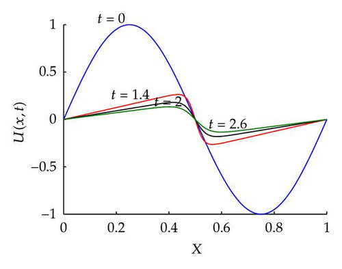
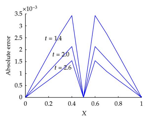
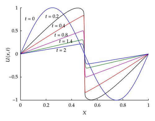
From Table 2, we find that the accuracy measured in L2, L∞ and RMS norm errors increases as the step size decrease. The numerical solutions are in the symmetric pattern as the exact solutions are. Table 3 and Figure 1 show a comparison between numerical and exact solutions at different times for ν = 0.005. The curves for distribution of absolute errors at different times are also shown in Figure 2. It is known that the Fourier solutions for ν ≤ 0.001 fail to converge because of the slow convergence of the infinite series [28]. The numerical solution cures for ν = 0.001 at different time are drawn in Figure 3, which shows the correct physical behavior.
| x | Numerical solution | Exact solution | ||
|---|---|---|---|---|
| N = 10 | N = 20 | N = 100 | ||
| 0.1 | 0.00847 | 0.01059 | 0.01129 | 0.01132 |
| 0.2 | 0.01370 | 0.01715 | 0.01828 | 0.01833 |
| 0.3 | 0.01371 | 0.01716 | 0.01830 | 0.01835 |
| 0.4 | 0.00848 | 0.01061 | 0.01132 | 0.01135 |
| 0.5 | 0.00000 | 0.00000 | 0.00000 | 0.00000 |
| 0.6 | −0.00848 | −0.01061 | −0.01132 | −0.01135 |
| 0.7 | −0.01371 | −0.01716 | −0.01830 | −0.01835 |
| 0.8 | −0.01370 | −0.01715 | −0.01829 | −0.01833 |
| 0.9 | −0.00847 | −0.01059 | −0.01129 | −0.01132 |
| N | ∥e∥RMS | ||
|---|---|---|---|
| 10 | 1.089E − 02 | 2.789E − 03 | 1.125E − 04 |
| 20 | 4.640E − 03 | 1.190E − 03 | 5.000E − 05 |
| 100 | 3.631E − 03 | 9.296E − 04 | 3.756E − 05 |
| x | t | |||||
|---|---|---|---|---|---|---|
| 1.4 | 2.0 | 2.6 | ||||
| Numerical | Exact | Numerical | Exact | Numerical | Exact | |
| 0.1 | 0.06303 | 0.06394 | 0.04567 | 0.04621 | 0.03581 | 0.03618 |
| 0.2 | 0.11975 | 0.12784 | 0.09133 | 0.09241 | 0.07162 | 0.07234 |
| 0.3 | 0.18902 | 0.19168 | 0.13694 | 0.13854 | 0.10717 | 0.10826 |
| 0.4 | 0.25091 | 0.25434 | 0.17809 | 0.18022 | 0.13367 | 0.13521 |
| 0.5 | 0.00000 | 0.00000 | 0.00000 | 0.00000 | 0.00000 | 0.00000 |
| 0.6 | −0.25091 | −0.25434 | −0.17809 | −0.18022 | −0.13367 | −0.13521 |
| 0.7 | −0.18902 | −0.19168 | −0.13694 | −0.13854 | −0.10717 | −0.10826 |
| 0.8 | −0.12605 | −0.12784 | −0.09133 | −0.09241 | −0.07162 | −0.07234 |
| 0.9 | −0.06303 | −0.06394 | −0.04567 | −0.04621 | −0.03581 | −0.03618 |
Example 4.2. Consider Burgers equation with the following forms:
It possesses the exact solution [23]
In the computation, we compare the result with the D1Q2 and D1Q3 lattice Boltzmann model whose equilibrium distribution functions are taken as
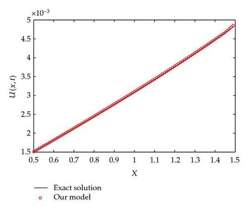
Let Re = 500, we give the results of our model, and exact solution as Figure 4 at t = 0.4. Table 4 shows the results of the D1Q2, D1Q3, our model and the exact solution at different lattice at time t = 0.4. The global relative errors
From Figure 4 and Table 4, we find that the D1Q2, D1Q3, and our model are all in excellent agreement with the exact solutions. The accuracy of the multilevel finite difference model is even higher than the D1Q2 and D1Q3 model. It should be pointed out that in order to attain better accuracy, the LB model requires a relatively small time step Δt but the multilevel finite difference model does not have this restriction.
| x | D1Q2 model | D1Q3 model | Our model | Exact solution |
|---|---|---|---|---|
| 0.5 | 0.001500 | 0.001500 | 0.001500 | 0.001500 |
| 0.6 | 0.001795 | 0.001787 | 0.001788 | 0.001786 |
| 0.7 | 0.002112 | 0.002099 | 0.002103 | 0.002096 |
| 0.8 | 0.002431 | 0.002414 | 0.002420 | 0.002411 |
| 0.9 | 0.002755 | 0.002734 | 0.002742 | 0.002731 |
| 1.0 | 0.003086 | 0.003060 | 0.003069 | 0.003056 |
| 1.1 | 0.003425 | 0.003393 | 0.003402 | 0.003389 |
| 1.2 | 0.003773 | 0.003735 | 0.003742 | 0.003729 |
| 1.3 | 0.004131 | 0.004087 | 0.004092 | 0.004080 |
| 1.4 | 0.004511 | 0.004483 | 0.004451 | 0.004421 |
| 1.5 | 0.005000 | 0.005000 | 0.005000 | 0.005000 |
| D1Q2 model | D1Q3 model | Our model | |
|---|---|---|---|
| GRE | 3.2383E − 03 | 1.7094E − 03 | 5.8823E − 04 |
5. Conclusion
In the current study, a three-level explicit finite difference scheme for 1D Burgers equation is derived by rewriting the LB scheme. Furthermore, it is proved that the scheme is conditionally stable. The efficiency and accuracy of the proposed scheme are validated through detail numerical simulation. It can be found that the numerical solutions are in excellent agreement with the analytical solutions. In order to derive LB scheme in a higher dimension, the LBM with the multispeed velocity model will be useful, in which different free parameters will be assigned for different values of the speed. Application of our method to 2D and 3D equations is left for future work.
Acknowledgments
This work was supported by the National Natural Science Foundation of China (no. 51174236) and National Basic Research Program of China (2011CB606306).


