Volume 2012, Issue 1 684074

Research Article

Open Access

Least-Squares Parameter Estimation Algorithm for a Class of Input Nonlinear Systems

Weili Xiong

Key Laboratory of Advanced Process Control for Light Industry of Ministry of Education, Jiangnan University, Wuxi 214122, China jiangnan.edu.cn

Search for more papers by this author

Wei Fan,

Wei Fan

School of Internet of Things Engineering, Jiangnan University, Wuxi 214122, China jiangnan.edu.cn

Search for more papers by this author

Rui Ding,

Corresponding Author

Rui Ding

[email protected]

School of Internet of Things Engineering, Jiangnan University, Wuxi 214122, China jiangnan.edu.cn

Search for more papers by this author

Weili Xiong,

Weili Xiong

Key Laboratory of Advanced Process Control for Light Industry of Ministry of Education, Jiangnan University, Wuxi 214122, China jiangnan.edu.cn

Search for more papers by this author

Wei Fan,

Wei Fan

School of Internet of Things Engineering, Jiangnan University, Wuxi 214122, China jiangnan.edu.cn

Search for more papers by this author

Rui Ding,

Corresponding Author

Rui Ding

[email protected]

School of Internet of Things Engineering, Jiangnan University, Wuxi 214122, China jiangnan.edu.cn

Search for more papers by this author

First published: 13 August 2012

https://doi.org/10.1155/2012/684074

Citations: 15

Academic Editor: Morteza Rafei

Share a link

Email
Wechat
Bluesky

Abstract

This paper studies least-squares parameter estimation algorithms for input nonlinear systems, including the input nonlinear controlled autoregressive (IN-CAR) model and the input nonlinear controlled autoregressive autoregressive moving average (IN-CARARMA) model. The basic idea is to obtain linear-in-parameters models by overparameterizing such nonlinear systems and to use the least-squares algorithm to estimate the unknown parameter vectors. It is proved that the parameter estimates consistently converge to their true values under the persistent excitation condition. A simulation example is provided.

1. Introduction

Parameter estimation has received much attention in many areas such as linear and nonlinear system identification and signal processing [1–9]. Nonlinear systems can be simply divided into the input nonlinear systems, the output nonlinear systems, the feedback nonlinear systems, and the input and output nonlinear systems, and so forth. The Hammerstein models can describe a class of input nonlinear systems which consist of static nonlinear blocks followed by linear dynamical subsystems [10, 11].

Nonlinear systems are common in industrial processes, for example, the dead-zone nonlinearities and the valve saturation nonlinearities. Many estimation methods have been developed to identify the parameters of nonlinear systems, especially for Hammerstein nonlinear systems [12, 13]. For example, Ding et al. presented a least-squares-based iterative algorithm and a recursive extended least squares algorithm for Hammerstein ARMAX systems [14] and an auxiliary model-based recursive least squares algorithm for Hammerstein output error systems [15]. Wang and Ding proposed an extended stochastic gradient identification algorithm for Hammerstein-Wiener ARMAX Systems [16].

Recently, Wang et al. derived an auxiliary model-based recursive generalized least-squares parameter estimation algorithm for Hammerstein output error autoregressive systems and auxiliary model-based RELS and MI-ELS algorithms for Hammerstein output error moving average systems using the key term separation principle [17, 18]. Ding et al. presented a projection estimation algorithm and a stochastic gradient (SG) estimation algorithm for Hammerstein nonlinear systems by using the gradient search and further derived a Newton recursive estimation algorithm and a Newton iterative estimation algorithm by using the Newton method (Newton-Raphson method) [19]. Wang and Ding studied least-squares-based and gradient-based iterative identification methods for Wiener nonlinear systems [20].

Fan et al. discussed the parameter estimation problem for Hammerstein nonlinear ARX models [21]. On the basis of the work in [14, 15, 21], this paper studies the identification problems and their convergence for input nonlinear controlled autoregressive (IN-CAR) models using the martingale convergence theorem and gives the recursive generalized extended least-squares algorithm for input nonlinear controlled autoregressive autoregressive moving average (IN-CARARMA) models.

Briefly, the paper is organized as follows. Section 2 derives a linear-in-parameters identification model and gives a recursive least squares identification algorithm for input nonlinear CAR systems and analyzes the properties of the proposed algorithm. Section 4 gives the recursive generalized extended least squares algorithm for input nonlinear CARARMA systems. Section 5 provides an illustrative example to show the effectiveness of the proposed algorithms. Finally, we offer some concluding remarks in Section 6.

2. The Input Nonlinear CAR Model and Estimation Algorithm

Let us introduce some notations first. The symbol I (I_n) stands for an identity matrix of appropriate sizes (n × n); the superscript T denotes the matrix transpose; 1_n represents an n-dimensional column vector whose elements are 1; |X | = det [X] represents the determinant of the matrix X; the norm of a matrix X is defined by ∥X∥² = tr [XX^T]; λ_max[X] and λ_min[X] represent the maximum and minimum eigenvalues of the square matrix X, respectively; f(t) = o(g(t)) represents f(t)/g(t) → 0 as t → ∞; for g(t)⩾0, we write f(t) = O(g(t)) if there exists a positive constant δ₁ such that |f(t)| ⩽ δ₁g(t).

2.1. The Input Nonlinear CAR Model

Consider the following input nonlinear controlled autoregressive (IN-CAR) systems [14, 21]:

()

where y(t) is the system output, v(t) is a disturbance noise, the output of the nonlinear block

is a nonlinear function of a known basis (f₁, f₂, …, f_m) of the system input u(t) [19],

()

A(z) and B(z) are polynomials in the unit backward shift operator z⁻¹ [z⁻¹y(t) = y(t − 1)], defined as

()

In order to obtain the identifiability of parameters b_i and c_i, without loss of generality, we suppose that c₁ = 1 or b₁ = 1 [14, 21].

Define the parameter vector ϑ and information vector ψ(t) as

()

From (2.1), we have

()

An alternative way is to define the parameter vector θ and information vector φ(t) as

()

Then (2.5) can be written as

()

Equations (2.6) and (2.8) are both linear-in-parameters identification model for Hammerstein CAR systems by using parametrization.

2.2. The Recursive Least Squares Algorithm

Minimizing the cost function

()

gives the following recursive least squares algorithm for computing the estimate

of θ in (2.8):

()

Applying the matrix inversion formula [22]

()

to (2.11) and defining the gain vector

, the algorithm in (2.10)-(2.11) can be equivalently expressed as

()

To initialize the algorithm, we take p₀ to be a large positive real number, for example, p₀ = 10⁶, and

to be some small real vector, for example,

3. The Main Convergence Theorem

The following lemmas are required to establish the main convergence results.

Lemma 3.1 (Martingale convergence theorem: Lemma D.5.3 in [23, 24]). If T_t, α_t, β_t are nonnegative random variables, measurable with respect to a nondecreasing sequence of σ algebra ℱ_t−1, and satisfy

()

then when

, one has

and T_t → T, a.s. (a.s.: almost surely) a finite nonnegative random variable.

Lemma 3.2 (see [14], [21], [25].)For the algorithm in (2.10)-(2.11), for any γ > 1, the covariance matrix P(t) in (2.11) satisfies the following inequality:

()

Theorem 3.3. For the system in (2.8) and the algorithm in (2.10)-(2.11), assume that {v(t), ℱ_t} is a martingale difference sequence defined on a probability space {Ω, ℱ, P}, where {ℱ_t} is the σ algebra sequence generated by the observations {y(t), y(t − 1), …, u(t), u(t − 1), …} and the noise sequence {v(t)} satisfies E[v(t)∣ℱ_t−1] = 0, and E[v²(t)∣ℱ_t−1] ⩽ σ² < ∞, a.s [23], and , γ > 1. Then the parameter estimation error converges to zero.

Proof. Define the parameter estimation error vector and the stochastic Lyapunov function . Let . According to the definitions of and T(t) and using (2.10) and (2.11), we have

()

Here, we have used the inequality 1 − φ^T(t)P(t)φ(t) = [1 + φ^T(t)P(t − 1)φ(t)] ⁻¹⩾0. Because

and φ^T(t)P(t)φ(t) are uncorrelated with v(t) and are ℱ_t−1 measurable, taking the conditional expectation with respect to ℱ_t−1, we have

()

Since ln | P⁻¹(t)| is nondecreasing, letting

()

we have

()

Using Lemma 3.2, the sum of the last term in the right-hand side for t from 1 to ∞ is finite. Applying Lemma 3.1 to the previous inequality, we conclude that V(t) converges a.s. to a finite random variable, say V₀, that is:

()

Thus, according to the definition of T(t), we have

()

This completes the proof of Theorem 3.3.

According to the definition of θ and the assumption b₁ = 1, the estimates

and

, …,

of a and c can be read from the first n and second m entries of

, respectively. Let

be the ith element of

. Referring to the definition of θ, the estimates

of b_j, j = 2,3, …, n, may be computed by

()

Notice that there is a large amount of redundancy about

for each i = 1,2, …, m. Since we do not need such m estimates

, one way is to take their average as the estimate of b_j [14], that is:

()

4. The Input Nonlinear CARARMA System and Estimation Algorithm

Consider the following input nonlinear controlled autoregressive autoregressive moving average (IN-CARARMA) systems:

()

Let

()

Define the parameter vector θ and information vector φ(t) as

()

Then (4.1) can be written as

()

This is a linear-in-parameter identification model for IN-CARARMA systems.

The unknown w(t − i) and v(t − i) in the information vector φ(t) are replaced with their estimates

and

, and then we can obtain the following recursive generalized extended least squares algorithm for estimating θ in (4.6):

()

This paper presents a recursive least squares algorithm for IN-CAR systems and a recursive generalized extended least squares algorithm for IN-CARARMA systems with ARMA noise disturbances, which differ not only from the input nonlinear controlled autoregressive moving average (IN-CARMA) systems in [14] but also from the input nonlinear output error systems in [15].

5. Example

Consider the following IN-CAR system:

()

In simulation, the input {u(t)} is taken as a persistent excitation signal sequence with zero mean and unit variance and {v(t)} as a white noise sequence with zero mean and constant variance σ². Applying the proposed algorithm in (2.10)-(2.11) to estimate the parameters of this system, the parameter estimates θ and θ_s and their errors with different noise variances are shown in Tables 1, 2, 3, and 4, and the parameter estimation errors

and

versus t are shown in Figures 1 and 2. When σ² = 0.50² and σ² = 1.50², the corresponding noise-to-signal ratios are δ_ns = 10.96% and δ_ns = 32.87%, respectively.

Table 1. The parameter estimates (θ) (σ² = 0.50², δ_ns = 10.96%).

t	a₁	a₂	c₁	c₂	c₃	b₂c₁	b₂c₂	b₂c₃	δ (%)
100	−1.35989	0.76938	0.94139	0.49861	0.18862	1.69875	0.86164	0.32773	2.59527
200	−1.35622	0.76001	0.96720	0.50101	0.19076	1.67233	0.84941	0.34369	1.43552
500	−1.35239	0.75452	1.00256	0.50137	0.19363	1.66468	0.84394	0.34485	0.74281
1000	−1.35034	0.75193	1.00570	0.50128	0.19460	1.65482	0.85095	0.33765	1.06112
2000	−1.34844	0.74940	0.99224	0.50089	0.20143	1.69169	0.85148	0.33583	0.67584
3000	−1.34776	0.74847	0.99012	0.49943	0.20333	1.68675	0.85321	0.33416	0.68173

True values	−1.35000	0.75000	1.00000	0.50000	0.20000	1.68000	0.84000	0.33600

Table 2. The parameter estimates (θ _s) (σ² = 0.50², δ_ns = 10.96%).

t	a₁	a₂	b₂	c₁	c₂	c₃	δ (%)
100	−1.35989	0.76938	1.75670	0.94139	0.49861	0.18862	3.90775
200	−1.35622	0.76001	1.74205	0.96720	0.50101	0.19076	2.81582
500	−1.35239	0.75452	1.70821	1.00256	0.50137	0.19363	1.15783
1000	−1.35034	0.75193	1.69268	1.00570	0.50128	0.19460	0.59233
2000	−1.34844	0.74940	1.69068	0.99224	0.50089	0.20143	0.52605
3000	−1.34776	0.74847	1.68512	0.99012	0.49943	0.20333	0.46851

True values	−1.35000	0.75000	1.68000	1.00000	0.50000	0.20000

Table 3. The parameter estimates (θ ) (σ² = 1.50², δ_ns = 32.87%).

t	a₁	a₂	c₁	c₂	c₃	b₂c₁	b₂c₂	b₂c₃	δ (%)
100	−1.37143	0.79561	0.81731	0.49688	0.16665	1.75280	0.90056	0.30999	7.98804
200	−1.36256	0.77335	0.89403	0.50353	0.17365	1.65999	0.87041	0.36082	4.46419
500	−1.35374	0.76009	1.00710	0.50417	0.18108	1.63863	0.85315	0.36321	2.08028
1000	−1.35074	0.75537	1.01710	0.50372	0.18381	1.60488	0.87297	0.34101	3.17034
2000	−1.34587	0.74895	0.97678	0.50296	0.20424	1.71432	0.87455	0.33540	2.01031
3000	−1.34448	0.74649	0.97053	0.49834	0.20990	1.69896	0.87916	0.33025	2.00404

True values	−1.35000	0.75000	1.00000	0.50000	0.20000	1.68000	0.84000	0.33600

Table 4. The parameter estimates (θ _s) (σ² = 1.50², δ_ns = 32.87%).

t	a₁	a₂	b₂	c₁	c₂	c₃	δ (%)
100	−1.37143	0.79561	1.93906	0.81731	0.49688	0.16665	12.66088
200	−1.36256	0.77335	1.88773	0.89403	0.50353	0.17365	9.26624
500	−1.35374	0.76009	1.77500	1.00710	0.50417	0.18108	3.83703
1000	−1.35074	0.75537	1.72205	1.01710	0.50372	0.18381	1.90836
2000	−1.34587	0.74895	1.71204	0.97678	0.50296	0.20424	1.57452
3000	−1.34448	0.74649	1.69603	0.97053	0.49834	0.20990	1.39744

True values	−1.35000	0.75000	1.68000	1.00000	0.50000	0.20000

Details are in the caption following the image — **Figure 1**
Open in figure viewer PowerPoint

The parameter estimation errors δ versus t.

From Tables 1–4 and Figures 1 and 2, we can draw the following conclusions.

(i)
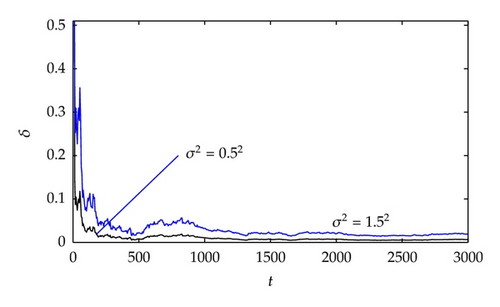
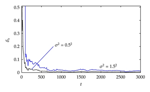
The larger the data length is, the smaller the parameter estimation errors become.
(ii)
A lower noise level leads to smaller parameter estimation errors for the same data length.
(iii)
The estimation errors δ and δ_s become smaller (in general) as t increases. This confirms the proposed theorem.

6. Conclusions

The recursive least-squares identification is used to estimate the unknown parameters for input nonlinear CAR and CARARMA systems. The analysis using the martingale convergence theorem indicates that the proposed recursive least squares algorithm can give consistent parameter estimation. It is worth pointing out that the multi-innovation identification theory [26–33], the gradient-based or least-squares-based identification methods [34–41], and other identification methods [42–49] can be used to study identification problem of this class of nonlinear systems with colored noises.

Acknowledgment

This work was supported by the 111 Project (B12018).

References

1 Zakerzadeh M. R., Firouzi M., Sayyaadi H., and Shouraki S. B., Hysteresis nonlinearity identification using new Preisach model-based artificial neural network approach, Journal of Applied Mathematics. (2011) 22, 458768, https://doi.org/10.1155/2011/458768, 2788363, ZBL1215.93037.
10.1155/2011/458768
Google Scholar
2 Li X.-X., Guo H. Z., Wan S. M., and Yang F., Inverse source identification by the modified regularization method on poisson equation, Journal of Applied Mathematics. (2012) 2012, 13, 971952, 2-s2.0-84856501573, https://doi.org/10.1155/2012/971952.
10.1155/2012/971952
Google Scholar
3 Shi Y. and Fang H., Kalman filter-based identification for systems with randomly missing measurements in a network environment, International Journal of Control. (2010) 83, no. 3, 538–551, https://doi.org/10.1080/00207170903273987, 2642903, ZBL1222.93228.
10.1080/00207170903273987
Web of Science® Google Scholar
4 Liu Y., Sheng J., and Ding R., Convergence of stochastic gradient estimation algorithm for multivariable ARX-like systems, Computers & Mathematics with Applications. (2010) 59, no. 8, 2615–2627, https://doi.org/10.1016/j.camwa.2010.01.030, 2607966, ZBL1193.60057.
10.1016/j.camwa.2010.01.030
Web of Science® Google Scholar
5 Ding F., Liu G., and Liu X. P., Parameter estimation with scarce measurements, Automatica. (2011) 47, no. 8, 1646–1655, 2-s2.0-79960912040.
10.1016/j.automatica.2011.05.007
Web of Science® Google Scholar
6 Ding J., Ding F., Liu X. P., and Liu G., Hierarchical least squares identification for linear SISO systems with dual-rate sampled-data, IEEE Transactions on Automatic Control. (2011) 56, no. 11, 2677–2683, https://doi.org/10.1109/TAC.2011.2158137, 2884009.
10.1109/TAC.2011.2158137
Web of Science® Google Scholar
7 Liu Y., Xiao Y., and Zhao X., Multi-innovation stochastic gradient algorithm for multiple-input single-output systems using the auxiliary model, Applied Mathematics and Computation. (2009) 215, no. 4, 1477–1483, https://doi.org/10.1016/j.amc.2009.07.012, 2571635, ZBL1177.65095.
10.1016/j.amc.2009.07.012
Web of Science® Google Scholar
8 Ding J. and Ding F., The residual based extended least squares identification method for dual-rate systems, Computers & Mathematics with Applications. (2008) 56, no. 6, 1479–1487, https://doi.org/10.1016/j.camwa.2008.02.047, 2440565, ZBL1155.93435.
10.1016/j.camwa.2008.02.047
Web of Science® Google Scholar
9 Han L. and Ding F., Identification for multirate multi-input systems using the multi-innovation identification theory, Computers & Mathematics with Applications. (2009) 57, no. 9, 1438–1449, https://doi.org/10.1016/j.camwa.2009.01.005, 2509957, ZBL1186.93076.
10.1016/j.camwa.2009.01.005
Web of Science® Google Scholar
10 Ding F., Shi Y., and Chen T., Gradient-based identification methods for Hammerstein nonlinear ARMAX models, Nonlinear Dynamics. (2006) 45, no. 1-2, 31–43, https://doi.org/10.1007/s11071%2D005%2D1850%2Dz, 2251164, ZBL1134.93321.
10.1007/s11071-005-1850-z
Web of Science® Google Scholar
11 Ding F., Chen T., and Iwai Z., Adaptive digital control of Hammerstein nonlinear systems with limited output sampling, SIAM Journal on Control and Optimization. (2007) 45, no. 6, 2257–2276, https://doi.org/10.1137/05062620X, 2285723, ZBL1126.93034.
10.1137/05062620X
Web of Science® Google Scholar
12 Li J. and Ding F., Maximum likelihood stochastic gradient estimation for Hammerstein systems with colored noise based on the key term separation technique, Computers & Mathematics with Applications. (2011) 62, no. 11, 4170–4177, https://doi.org/10.1016/j.camwa.2011.09.067, 2859972.
10.1016/j.camwa.2011.09.067
Web of Science® Google Scholar
13 Li J., Ding F., and Yang G., Maximum likelihood least squares identification method for input nonlinear finite impulse response moving average systems, Mathematical and Computer Modelling. (2012) 55, no. 3-4, 442–450, 2-s2.0-80755154802, https://doi.org/10.1016/j.mcm.2011.08.023.
10.1016/j.mcm.2011.08.023
Google Scholar
14 Ding F. and Chen T., Identification of Hammerstein nonlinear ARMAX systems, Automatica. (2005) 41, no. 9, 1479–1489, https://doi.org/10.1016/j.automatica.2005.03.026, 2161111, ZBL1086.93063.
10.1016/j.automatica.2005.03.026
Web of Science® Google Scholar
15 Ding F., Shi Y., and Chen T., Auxiliary model-based least-squares identification methods for Hammerstein output-error systems, Systems & Control Letters. (2007) 56, no. 5, 373–380, https://doi.org/10.1016/j.sysconle.2006.10.026, 2311199, ZBL1130.93055.
10.1016/j.sysconle.2006.10.026
Web of Science® Google Scholar
16 Wang D. and Ding F., Extended stochastic gradient identification algorithms for Hammerstein-Wiener ARMAX systems, Computers & Mathematics with Applications. (2008) 56, no. 12, 3157–3164, https://doi.org/10.1016/j.camwa.2008.07.015, 2474571, ZBL1165.65308.
10.1016/j.camwa.2008.07.015
Web of Science® Google Scholar
17 Wang D., Chu Y., Yang G., and Ding F., Auxiliary model based recursive generalized least squares parameter estimation for Hammerstein OEAR systems, Mathematical and Computer Modelling. (2010) 52, no. 1-2, 309–317, https://doi.org/10.1016/j.mcm.2010.03.002, 2645942, ZBL1201.93134.
10.1016/j.mcm.2010.03.002
Google Scholar
18 Wang D., Chu Y., and Ding F., Auxiliary model-based RELS and MI-ELS algorithm for Hammerstein OEMA systems, Computers & Mathematics with Applications. (2010) 59, no. 9, 3092–3098, https://doi.org/10.1016/j.camwa.2010.02.030, 2610541, ZBL1193.93170.
10.1016/j.camwa.2010.02.030
Web of Science® Google Scholar
19 Ding F., Liu X. P., and Liu G., Identification methods for Hammerstein nonlinear systems, Digital Signal Processing. (2011) 21, no. 2, 215–238, 2-s2.0-79551472381, https://doi.org/10.1016/j.dsp.2010.06.006.
10.1016/j.dsp.2010.06.006
Web of Science® Google Scholar
20 Wang D. and Ding F., Least squares based and gradient based iterative identification for Wiener nonlinear systems, Signal Processing. (2011) 91, no. 5, 1182–1189, 2-s2.0-79551473739, https://doi.org/10.1016/j.sigpro.2010.11.004.
10.1016/j.sigpro.2010.11.004
Web of Science® Google Scholar
21 Fan W., Ding F., and Shi Y., Parameter estimation for Hammerstein nonlinear controlled auto-regression models, Proceedings of the IEEE International Conference on Automation and Logistics, August 2007, Jinan, China, 1007–1012.
Google Scholar
22 Wang L., Ding F., and Liu P. X., Convergence of HLS estimation algorithms for multivariable ARX-like systems, Applied Mathematics and Computation. (2007) 190, no. 2, 1081–1093, https://doi.org/10.1016/j.amc.2007.01.089, 2339702, ZBL1117.93332.
10.1016/j.amc.2007.01.089
Web of Science® Google Scholar
23 Goodwin G. C. and Sin K. S., Adaptive Filtering, Prediction and Control, 1984, Prentice-Hall, Englewood Cliffs, NJ, USA.
Google Scholar
24 Liu Y., Yu L., and Ding F., Multi-innovation extended stochastic gradient algorithm and its performance analysis, Circuits, Systems, and Signal Processing. (2010) 29, no. 4, 649–667, https://doi.org/10.1007/s00034%2D010%2D9174%2D8, 2658246, ZBL1196.94026.
10.1007/s00034-010-9174-8
Web of Science® Google Scholar
25 Ding F. and Chen T., Combined parameter and output estimation of dual-rate systems using an auxiliary model, Automatica. (2004) 40, no. 10, https://doi.org/10.1016/j.automatica.2004.05.001, 2155466, ZBL1162.93376.
10.1016/j.automatica.2004.05.001
Web of Science® Google Scholar
26 Ding F. and Chen T., Performance analysis of multi-innovation gradient type identification methods, Automatica. (2007) 43, no. 1, 1–14, https://doi.org/10.1016/j.automatica.2006.07.024, 2266765, ZBL1140.93488.
10.1016/j.automatica.2006.07.024
CAS Web of Science® Google Scholar
27 Han L. and Ding F., Multi-innovation stochastic gradient algorithms for multi-input multi-output systems, Digital Signal Processing. (2009) 19, no. 4, 545–554, 2-s2.0-67349090936, https://doi.org/10.1016/j.dsp.2008.12.002.
10.1016/j.dsp.2008.12.002
Web of Science® Google Scholar
28 Ding F., Several multi-innovation identification methods, Digital Signal Processing. (2010) 20, no. 4, 1027–1039.
10.1016/j.dsp.2009.10.030
Web of Science® Google Scholar
29 Wang D. and Ding F., Performance analysis of the auxiliary models based multi-innovation stochastic gradient estimation algorithm for output error systems, Digital Signal Processing. (2010) 20, no. 3, 750–762, 2-s2.0-77949486033, https://doi.org/10.1016/j.dsp.2009.09.002.
10.1016/j.dsp.2009.09.002
Web of Science® Google Scholar
30 Zhang J., Ding F., and Shi Y., Self-tuning control based on multi-innovation stochastic gradient parameter estimation, Systems & Control Letters. (2009) 58, no. 1, 69–75, https://doi.org/10.1016/j.sysconle.2008.08.005, 2488777, ZBL1154.93040.
10.1016/j.sysconle.2008.08.005
Web of Science® Google Scholar
31 Ding F., Chen H., and Li M., Multi-innovation least squares identification methods based on the auxiliary model for MISO systems, Applied Mathematics and Computation. (2007) 187, no. 2, 658–668, https://doi.org/10.1016/j.amc.2006.08.090, 2323072, ZBL1114.93101.
10.1016/j.amc.2006.08.090
Web of Science® Google Scholar
32 Xie L., Liu Y. J., Yang H. Z., and Ding F., Modelling and identification for non-uniformly periodically sampled-data systems, IET Control Theory & Applications. (2010) 4, no. 5, 784–794, https://doi.org/10.1049/iet%2Dcta.2009.0064, 2758794.
10.1049/iet-cta.2009.0064
Web of Science® Google Scholar
33 Ding F., Liu P. X., and Liu G., Multiinnovation least-squares identification for system modeling, IEEE Transactions on Systems, Man, and Cybernetics B. (2010) 40, no. 3, 767–778, 5299173, 2-s2.0-77952585183, https://doi.org/10.1109/TSMCB.2009.2028871.
10.1109/TSMCB.2009.2028871
PubMed Web of Science® Google Scholar
34 Ding J., Shi Y., Wang H., and Ding F., A modified stochastic gradient based parameter estimation algorithm for dual-rate sampled-data systems, Digital Signal Processing. (2010) 20, no. 4, 1238–1247, 2-s2.0-77954174918, https://doi.org/10.1016/j.dsp.2009.10.023.
10.1016/j.dsp.2009.10.023
Web of Science® Google Scholar
35 Ding F., Liu P. X., and Yang H., Parameter identification and intersample output estimation for dual-rate systems, IEEE Transactions on Systems, Man, and Cybernetics A. (2008) 38, no. 4, 966–975, 2-s2.0-46649118857, https://doi.org/10.1109/TSMCA.2008.923030.
10.1109/TSMCA.2008.923030
Web of Science® Google Scholar
36 Liu Y., Wang D., and Ding F., Least squares based iterative algorithms for identifying Box-Jenkins models with finite measurement data, Digital Signal Processing. (2010) 20, no. 5, 1458–1467, 2-s2.0-77954174851, https://doi.org/10.1016/j.dsp.2010.01.004.
10.1016/j.dsp.2010.01.004
Web of Science® Google Scholar
37 Wang D. and Ding F., Input-output data filtering based recursive least squares identification for CARARMA systems, Digital Signal Processing. (2010) 20, no. 4, 991–999, 2-s2.0-77954175887, https://doi.org/10.1016/j.dsp.2009.12.006.
10.1016/j.dsp.2009.12.006
Web of Science® Google Scholar
38 Ding F., Liu P. X., and Liu G., Gradient based and least-squares based iterative identification methods for OE and OEMA systems, Digital Signal Processing. (2010) 20, no. 3, 664–677, 2-s2.0-77949486667, https://doi.org/10.1016/j.dsp.2009.10.012.
10.1016/j.dsp.2009.10.012
Web of Science® Google Scholar
39 Wang D., Yang G., and Ding R., Gradient-based iterative parameter estimation for Box-Jenkins systems, Computers & Mathematics with Applications. (2010) 60, no. 5, 1200–1208, https://doi.org/10.1016/j.camwa.2010.06.001, 2672919, ZBL1201.94046.
10.1016/j.camwa.2010.06.001
PubMed Web of Science® Google Scholar
40 Xie L., Yang H., and Ding F., Recursive least squares parameter estimation for non-uniformly sampled systems based on the data filtering, Mathematical and Computer Modelling. (2011) 54, no. 1-2, 315–324, https://doi.org/10.1016/j.mcm.2011.02.014, 2801888, ZBL1225.62120.
10.1016/j.mcm.2011.02.014
Web of Science® Google Scholar
41 Ding F., Liu Y., and Bao B., Gradient-based and least-squares-based iterative estimation algorithms for multi-input multi-output systems, Proceedings of the Institution of Mechanical Engineers. Part I: Journal of Systems and Control Engineering. (2012) 226, no. 1, 43–55, 2-s2.0-84856298642, https://doi.org/10.1177/0959651811409491.
10.1177/0959651811409491
Web of Science® Google Scholar
42 Ding F., Hierarchical multi-innovation stochastic gradient algorithm for Hammerstein nonlinear system modeling, Applied Mathematical Modelling. In presshttps://doi.org/10.1016/j.apm.2012.04.039.
10.1016/j.apm.2012.04.039
Google Scholar
43 Ding F. and Ding J., Least-squares parameter estimation for systems with irregularly missing data, International Journal of Adaptive Control and Signal Processing. (2010) 24, no. 7, 540–553, https://doi.org/10.1002/acs.1141, 2680718, ZBL1200.93130.
10.1002/acs.1141
Web of Science® Google Scholar
44 Liu Y., Xie L., and Ding F., An auxiliary model based on a recursive least-squares parameter estimation algorithm for non-uniformly sampled multirate systems, Proceedings of the Institution of Mechanical Engineers. Part I: Journal of Systems and Control Engineering. (2009) 223, no. 4, 445–454, 2-s2.0-67650315437, https://doi.org/10.1243/09596518JSCE686.
10.1243/09596518JSCE686
Web of Science® Google Scholar
45 Ding F., Qiu L., and Chen T., Reconstruction of continuous-time systems from their non-uniformly sampled discrete-time systems, Automatica. (2009) 45, no. 2, 324–332, https://doi.org/10.1016/j.automatica.2008.08.007, 2527328, ZBL1158.93365.
10.1016/j.automatica.2008.08.007
Web of Science® Google Scholar
46 Ding F., Liu G., and Liu X. P., Partially coupled stochastic gradient identification methods for non-uniformly sampled systems, IEEE Transactions on Automatic Control. (2010) 55, no. 8, 1976–1981, https://doi.org/10.1109/TAC.2010.2050713, 2681302.
10.1109/TAC.2010.2050713
Web of Science® Google Scholar
47 Ding J. and Ding F., Bias compensation-based parameter estimation for output error moving average systems, International Journal of Adaptive Control and Signal Processing. (2011) 25, no. 12, 1100–1111, 2-s2.0-80755182664, https://doi.org/10.1002/acs.1266.
10.1002/acs.1266
Web of Science® Google Scholar
48 Ding F. and Chen T., Performance bounds of forgetting factor least-squares algorithms for time-varying systems with finite meaurement data, IEEE Transactions on Circuits and Systems. I. Regular Papers. (2005) 52, no. 3, 555–566, https://doi.org/10.1109/TCSI.2004.842874, 2124325.
10.1109/TCSI.2004.842874
Web of Science® Google Scholar
49 Ding F. and Chen T., Hierarchical identification of lifted state-space models for general dual-rate systems, IEEE Transactions on Circuits and Systems. I. Regular Papers. (2005) 52, no. 6, 1179–1187, https://doi.org/10.1109/TCSI.2005.849144, 2147479.
10.1109/TCSI.2005.849144
Web of Science® Google Scholar

Citing Literature

All articles

Least-Squares Parameter Estimation Algorithm for a Class of Input Nonlinear Systems

Abstract

1. Introduction

2. The Input Nonlinear CAR Model and Estimation Algorithm

2.1. The Input Nonlinear CAR Model

2.2. The Recursive Least Squares Algorithm

3. The Main Convergence Theorem

4. The Input Nonlinear CARARMA System and Estimation Algorithm

5. Example

6. Conclusions

Acknowledgment

References

Citing Literature

Figures

References

Information

About Wiley Online Library

Help & Support

Opportunities

Connect with Wiley

Least-Squares Parameter Estimation Algorithm for a Class of Input Nonlinear Systems

Abstract

1. Introduction

2. The Input Nonlinear CAR Model and Estimation Algorithm

2.1. The Input Nonlinear CAR Model

2.2. The Recursive Least Squares Algorithm

3. The Main Convergence Theorem

4. The Input Nonlinear CARARMA System and Estimation Algorithm

5. Example

6. Conclusions

Acknowledgment

References

Citing Literature

Figures

References

Related

Information