A prey-predator model with Beddington-DeAngelis functional response and impulsive state feedback control is investigated. We obtain the sufficient conditions of the global asymptotical stability of the system without impulsive effects. By using the geometry theory of semicontinuous dynamic system and the method of successor function, we obtain the system with impulsive effects that has an order one periodic solution, and sufficient conditions for existence and stability of order one periodic solution are also obtained. Finally, numerical simulations are performed to illustrate our main results.

1. Introduction

The study of the dynamics of prey-predator system is one of the dominant subjects in both ecology and mathematical ecology due to the fact that predator-prey interaction is the fundamental structure in population dynamics. Many scholars have carried out the study of prey-predator system with various functional responses, such as Monod-type and Holling-type. It is well known that Beddington-DeAngelis functional response which was introduced by Beddington and DeAngelis et al. [1, 2] can avoid some of the singular behavior of ratio-dependent models at low densities and provide better description of predator feeding over a range of prey-predator abundances. Therefore, in this paper, we investigate prey-predator system with Beddington-DeAngelis functional response.

Impulsive differential equations have been widely used in various fields of applied sciences, for example, physics, ecology, and pest control. The majority of them just concern the system with impulses at fixed times [3–7]. However, in practical ecological system, the control measures (by poisoning or releasing the natural nenmy, etc.) are taken only when the amount of species reaches a threshold value, rather than the usual impulsive fixed-time control strategy. Impulsive state feedback equation is a powerful tool to manage these problems. Therefore, some researchers proposed the impulsive state feedback control models for population management [8–11].

Motivated by the above works, in this paper, we consider the following predator-prey system with Beddington-DeAngelis functional respose:

()

where

, r, K, α, β, γ, d, and k are positive constants and x(τ), y(τ) represent the population density of prey (pest) and predator (natural enemy) at time τ, respectively. r is the intrinsic growth rate and K is the carrying capacity in the absence of predation. The predator consumes the prey with functional response of Beddington-DeAngelis type

and contributes to its growth with rate

. d is the death rate of predator. 0 < p < 1, 0 < q < 1, when the amount of the prey reaches the threshold h at time

, controlling measures are taken and the amount of the prey and predator abruptly turn to (1 − p)h₁ and

, respectively. The functional response in system (1.1) is similar to the well-known Holling type II with an extra term

in the denominator which models the mutual interference among predators. It also has some of the same qualitative behaviours as the classical ratio-dependent model (i.e., α = 0), but is free from the singular behaviors of ratio-dependent model at low densities which is, in fact, the source of controversy [12–14]. For simplicity, let

, then system (1.1) becomes the form:

()

We assume that k − dβ > 0, otherwise

, we have

as t → ∞, which means that the predator population will die out, therefore, in the following, we always assume that k − dβ > 0.

We nondimensionalize system (1.2) with the following scaling:

, and have

()

where the nondimensional parameters are defined as a₁ = (Kβ − α)d/(k − dβ)K, a₂ = 1 − (1/rγ), f = rα, e = αd, a₃ = αβd²/K(k − dβ) ², a₄ = αd/(k − dβ), h = ((k − dβ)/αd)h₁, and ι = (γ/α)ι₁. Obviously that e > 0, f > 0, a₃ > 0, a₄ > 0.

In this paper, we mainly discuss the existence and stability of periodic solution of system (1.3) by using the geometry theory of semicontinuous dynamic system and the method of successor function which were introduced in the paper [15, 16], as far as we know, there are few papers to apply these methods to prove the existence of order one periodic solution, which makes the study simpler and clearer. What is worth saying is that modeling thoughts and mathematical methods used in this paper are of more important theoretical and practical value.

An outline of this paper is as follows: some definitions and theorems are given for the later use in the next section. The qualitative analysis of the system without impulsive effects is given in Section 3. In Section 4, the existence and stability of order one periodic solution of system (1.3) are investigated. Numerical simulations and some discussions are provided in Section 5.

2. Definitions and Lemmas

Definition 2.1 (see [15].)Differential equation with impulsive state feedback control

()

where M{x, y} and N{x, y} are lines or curves on the plane R²(x, y). M{x, y} is called pulse set and N{x, y} is called phase set. The dynamical system which is constituted by the solution map of system (2.1) is called semicontinuous dynamical system which is denoted by (Ω, f, φ, M). We assume that the map with the initial point p is not in the pulse set M{x, y}, that is, p ∈ Ω = R² − M{x, y}, φ is a continuous map, φ(M)⊆N, and φ is called pulse map.

In this paper, R⁺ = [0, +∞), . , , , then system (1.3) constitutes a semicontinuous dynamical system (Ω, f, φ, M).

For any P ∈ Ω, the function f_P : R⁺ → Ω defined as f_P(t) = f(P, t) is continuous and we call f_P(t) the trajectory passing through point P. The set C⁺(P) = {f(P, t)∣0 ≤ t < +∞} is called positive semitrajectory of point P. The set C⁻(P) = {f(P, t)∣ − ∞ < t ≤ 0} is called the negative semitrajectory of point P. For the convenience, if P ∈ Ω, F(P) is defined as the first intersection point of C⁺(P) and M, that is, there exists a t₁ ∈ R⁺ such that F(P) = f(P, t₁) ∈ M, and for 0 < t < t₁, f(P, t) ∉ M.

Definition 2.2 (see [15].)A trajectory f(P, t) is called order one periodic solution with period T if there exists a point P ∈ N and T > 0 such that f(P, T) = Q ∈ M and φ(Q) = φ(f(P, T)) = P ∈ N.

Next we will give the definition of the successor function of semicontinuous dynamical system (1.3). First, we define a new number axis in set N. On straight line x = (1 − p)h, take the origin at point ((1 − p)h, 0) of coordinate axis x and define positive direction and unit length to be consistent with coordinate axis y, then we obtain a number axis l. For any x ∈ l, let l(x) be coordinate of point x.

Definition 2.3. Suppose g : N → N be a map. For any x ∈ N, there exists a t₁ > 0 such that F(x) = f(x, t₁) = x₁ ∈ M, , then is called the successor function of point x, and the point is called the successor point of x.

Remark 2.4. If g(x₀) = 0, the trajectory f(x₀, t) with initial point x₀ is an order one periodic solution of system (1.3).

According to the continuity of compound function, we know the following.

Lemma 2.5. The successor function g(x) is continuous.

In system (1.3), the isocline dx/dt = 0 is denoted by Γ₁, the isocline dy/dt = 0 is denoted by Γ₂. Let A((1 − p)h, y_A) be the intersection point of isocline Γ₁ and set N. If there exist two points x₁ ∈ N, x₂ ∈ N, which are both below A or above A, satisfying g(x₁)g(x₂) < 0, by the zero point theorem of continuous function in the closed interval, we know there exists a point x₀ ∈ N which is between x₁ and x₂ such that g(x₀) = 0, so we have the following.

Lemma 2.6 (existence theorem of order one periodic solution). The system (1.3) exists an order one periodic solution if there exist two points x₁ ∈ N, x₂ ∈ N, which are both below A or above A, satisfying g(x₁)g(x₂) < 0.

3. Qualitative Analysis of System (1.3) without Impulsive Effects

In this section, we will study the qualitative characteristic of system (1.3) without impulsive effects. If no impulsive effects is introduced, then system (1.3) is

()

The equilibrium of system (3.1) satisfies

()

It can be seen that system (3.1) exist boundary equilibrium O(0,0),

, where x₁ satisfied 1 + a₁x − a₃x² = 0 and a positive equilibrium B(x^*, y^*) provided that a₃ < 1 + a₁, a₂ < 0, where

, y^* = x^* − 1. In the following, we always suppose that a₁ < 0, a₂ < 0.

Lemma 3.1. The system (3.1) is uniformly bounded.

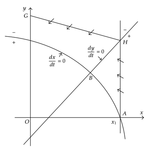
Proof. Let the straight line l₁ = x − x₁ = 0, we have , then the trajectory of system (3.1) from the right of l₁ through the l₁ into the left. Define a function V(x, y) = −(e/a₂)x + fy − K, where 0 < x < x₁. The function V(x, y) intersects the line x = x₁ and axis y at the points H and G, respectively. We have . we can choose K enough large such that dV/dt|_HG < 0. Hence, the system (3.1) is uniformly bounded (see Figure 1). The proof is completed.

Details are in the caption following the image — **Figure 1**
Open in figure viewer PowerPoint

The uniformly bounded region.

In the following, we will analysis the stability of equilibrium and B(S^*, x^*) of system (3.1). Clearly, O(0,0) is saddle point and if a₃ > 1 + a₁, is stable, otherwise is saddle point and the positive equilibrium point B(S^*, x^*) exists. For the positive equilibrium point, we have the following result.

Theorem 3.2. The positive equilibrium point B(S^*, x^*) is globally asymptotically stable if a₃ < 1 + a₁.

Proof. The Jacobian matrix J_B = J(x^*, y^*) of system (3.1) at B takes the form of

()

The eigenvalue problem for the J_B = J(x^*, y^*) provides the characteristic equation

()

where the coefficients Q₁, Q₂ are

()

Note that Q₁ > 0, Q₂ > 0, then both of the eigenvalues have negative real part, we have that B is locally asymptotically stable.

Let P(x, y) = fx(1 + a₁x + a₂y − a₃x² − a₄xy), Q(x, y) = ey(x − y − 1) and B = x^α−1y^β−1, where α = −a₁/(1 + a₁), β = αf/e, then we have

()

the system (3.1) has no closed trajectory, therefore B(S^*, x^*) is globally asymptotically stable. This completes the proof.

4. Existence and Stability of Periodic Solutions of System (1.3)

4.1. Existence of Order One Periodic Solution

In this section, we will investigate the existence of order one periodic solution of system (1.3) by using the method of successor function. Note that system (1.3) is a semicontinuous dynamical system, for convenience, any point C, let x_C denote its abscissa and y_C be its ordinate. If C = (h, y_C) ∈ M, then impulse occurs at point C, the impulsive function transfers the point C into C⁺. Without loss of generality, unless otherwise specified we assume the initial point of the trajectory lies in N. From discussion of Section 3, we know that B is globally asymptotically stable when a₃ < 1 + a₁. If h > x^*, (1 − p)h > x^*, all the solutions of system (1.3) tend to the equilibrium B after finite impulse, so we mainly pay attention to the case h < x^* or h > x^* and (1 − p)h < x^*.

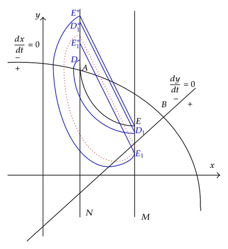
Case I (h < x*). In this case, sets M and N are both in the left side of point B. Trajectory passing through point A tangents to N at point A. Set F(A) = E(h, y_E) ∈ M, then impulse occurs at point E. Suppose point E is subject to impulsive effects to point , here , the position of E⁺ has the following three cases.

Case I₁ (). E⁺ coincides with A, and the successor function of A is , so trajectory and segment EA formulate an order one periodic solution of system (1.3).

Case I₂ (). In this case, E⁺ is above A. Set F(E⁺) = E₁ ∈ M, in view of vector field and disjointness of any two trajectories, we know , so we have , then the successor function of E⁺ is .

Take another point D((1 − p)h, y_A + ε) above A, where ε > 0 is small enough. Set F(D) = D₁ ∈ M, in view of continuous dependence of the solution on initial value and time, we know and the point D₁ is close to E enough, so we have and the point is close to E⁺ enough, since , then we obtain . By Lemma 2.6, we know there exists an order one periodic solution of system (1.3), whose initial point is between D and E⁺ in set N (see Figure 2).

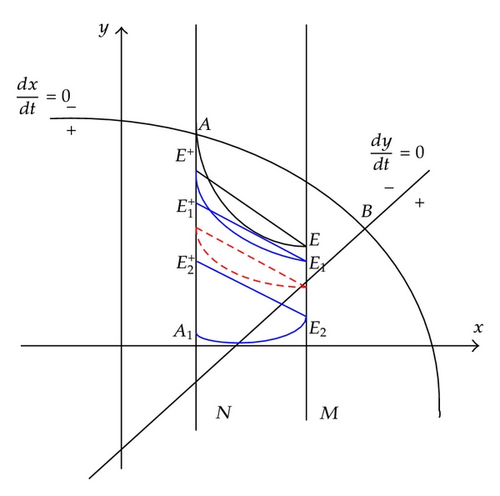
Case I₃ (). In this case, E⁺ is below A. We have , so , then the successor function of E⁺ is .

Take another point A₁((1 − p)h, ε) ∈ N satisfying 0 < ε < ι. Set F(A₁) = E₂ ∈ M, then , so we have . By Lemma 2.6, we know there exists an order one periodic solution of system (1.3), whose initial point is between E⁺ and A₁ in set N (see Figure 3). Therefore, we have the following theorem.

Theorem 4.1. Suppose that a₃ < 1 + a₁, h < x^*, then system (1.3) has an order one periodic solution.

Case II (h > x*, (1 − p)h < x*). In this case, set M is in the right side of B and set N in the left of B. Denote the intersection point of isocline Γ₁(dx/dt = 0) and set M by A(h, y_A). The trajectory passing through point A tangents to M at point A. G(x_h, y_h) is defined as the first intersection point of C⁻(A) and Γ₁, that is, there exists a T₁ > 0 such that f(A, −T₁) = G ∈ C⁻(A)⋂ Γ₁, and for −T₁ < t ≤ 0, f(A, t)⋂ Γ₁ = ∅.

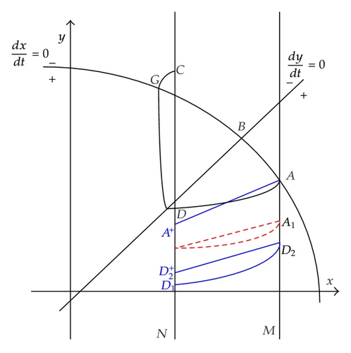
Case II₁ (x_G < (1 − p)h). There exist T₂, T₃ > 0 such that C ∈ C⁻(A)⋂ N, D ∈ C⁻(A)⋂ N, f(A, −T₂) = D, f(A, −T₃) = C, and for −T₃ < t < −T₂, f(A, t)⋂ N = ∅. Suppose point A is subject to impulsive effects to point .

If A⁺ coincides with C or D, trajectory and segment DA or trajectory and segment AC formulate an order one periodic solution of system (1.3).

If A⁺ is below D, that is, , the successor function of D is . Take another point D₁((1 − p)h, ε) ∈ N satisfying 0 < ε < ι. Set F(D₁) = D₂ ∈ M, then , then we have . We conclude that there exists an order one periodic solution of system (1.3), whose initial point is between D and D₁ in set N (see Figure 4).

If A⁺ is above C, that is, , the successor function of C is . Set F(A⁺) = A₁ ∈ M, in view of the vector fields of system (1.3), we know , so we have . We conclude that there exists an order one periodic solution of system (1.3), whose initial point is between C and A⁺ in set N (see Figure 5).

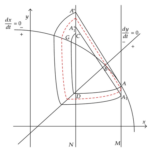
If A⁺ is between C and D, in view of vector fields, we know the trajectory of system (1.3) initiating any point between C and D of set N will be free from impulsive effects and ultimately tend to stable point B, thus there does not exist order one periodic solution in system (1.3) in this case. So we have the following.

Theorem 4.2. Suppose that a₃ < 1 + a₁, h > x^*, (1 − p)h < x^* and x_G < (1 − p)h, or , then system (1.3) has an order one periodic solution.

Case II₂ (x_G > (1 − p)h). Denote the intersection point of isocline Γ₁ and set N by K((1 − p)h, y_K). The trajectory passing through point K tangents to N at point K. Set F(K) = S(h, y_S) ∈ M, then impulse occurs at point S. Suppose point S is subject to impulsive effects to point . Like the analysis of Case I, we can prove that there exists an order one periodic solution in system (1.3) in this case (see Figure 6).

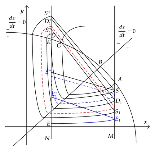
Theorem 4.3. Suppose that a₃ < 1 + a₁, h > x^*, (1 − p)h < x^* and x_G > (1 − p)h, then system (1.3) exists an order one periodic solution.

In the following, we analyze the stability of order one periodic solution in system (1.3). Firstly, we give one lemma to discuss the stability of this periodic solution of system (1.3).

Lemma 4.4. The T-periodic solution x = ξ(t), y = η(t) of the system,

()

is orbitally asymptotically stable if the Floquet multiplier μ₂ satisfies the condition |μ₂ | < 1, where

()

with

()

and P, Q, (∂α/∂x), (∂α/∂y), (∂β/∂x), (∂β/∂y), (∂ϕ/∂x), and (∂ϕ/∂y) are calculated at the point (ξ(τ_k), η(τ_k)),

. ϕ(x, y) is a sufficiently smooth function with grad ϕ(x, y) ≠ 0, and τ_k(k ∈ N) is the time of the kth jump.

The proof of this lemma is referred to Simeonov and Baĭnov [17].

In the following, we suppose this periodic solution of system (1.3) with period T passes through the points

, ι + (1 − q)η₀) ∈ N and H₁(h, η₀) ∈ M (see Figures 2–6). As the expression and the period of this solution are unknown, we discuss the stability of this positive periodic solution by Lemma 4.4. In our case,

()

Then

()

Set

()

if (x(t), y(t)) are period function with T, then

()

hence

()

Suppose H(t) = (∂P/∂x)(ξ(t), η(t)) + (∂Q/∂y)(ξ(t), η(t)), then

()

Because (ξ(t), η(t)) is period solution of system (1.3), we have

. Obviously, |μ₂ | < 1 if

()

Theorem 4.5. If system (1.3) has an order one periodic solution, this order one periodic solution is orbitally asymptotically stable provided

()

5. Numerical Analysis and Discussion

In order to verify the theoretical results in this paper, we consider the following example

()

In numerical simulation, let a₁ = −0.35, a₂ = −0.4, a₃ = 0.01, a₄ = 0.8, e = 0.4, and f = 0.5, by calculating we know a₃ < 1 + a₁, x^* = 1.34, y^* = 0.34. If h = 2.4 > x^*, p = 0.4, (1 − p)h = 1.44 > x^*, q = 0.5, ι = 0.8, then the time series and phase portrait can be seen in Figure 7, by analysis of Section 4, we know that in this case, system (1.3) has no periodic solution and all the solutions tend to the equilibrium B after finite impulses. If h = 1.2 < x^*, by Theorem 4.1, we know that system (1.3) has an order one periodic solution which is shown in Figure 8. As shown in Figure 9, if h = 1.4 > x^*, (1 − p)h = 0.84 < x^*, by Theorems 4.2 and 4.3, we know system (1.3) also has an order one periodic solution. The results show that prey-predator model with Beddington-DeAnglis functional response and impulsive state feedback control tends to stable state or be periodic, which means that the amount of prey is under control.

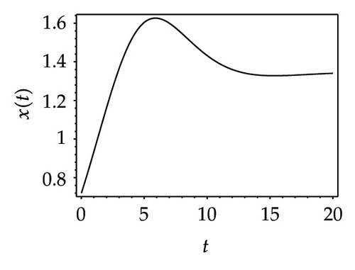
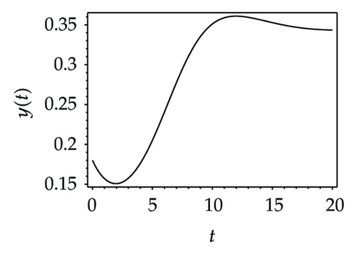
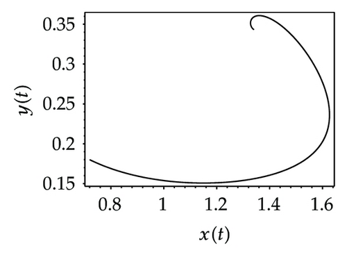
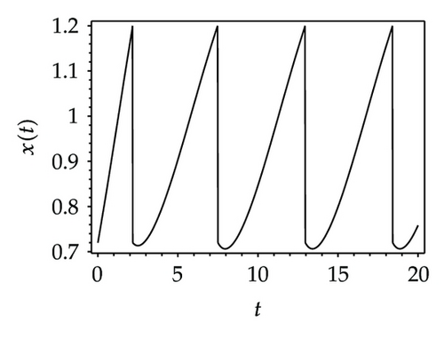
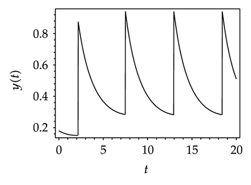
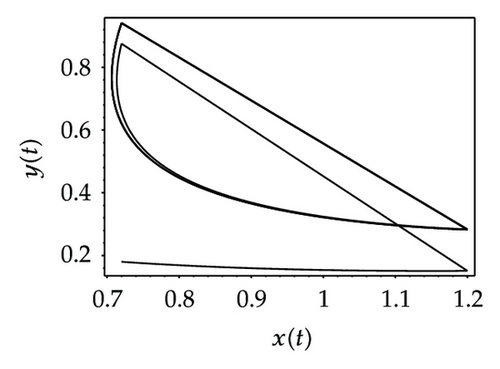
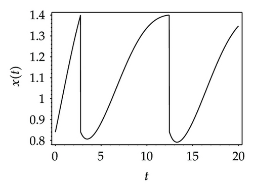
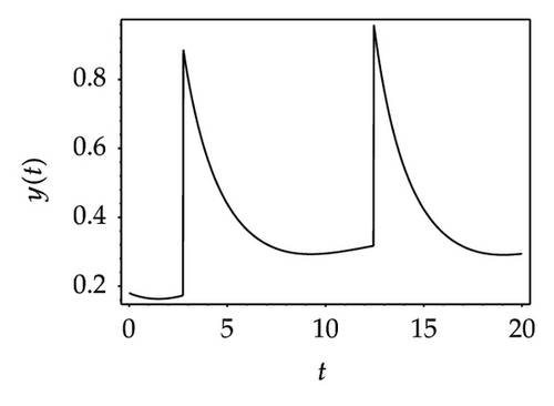
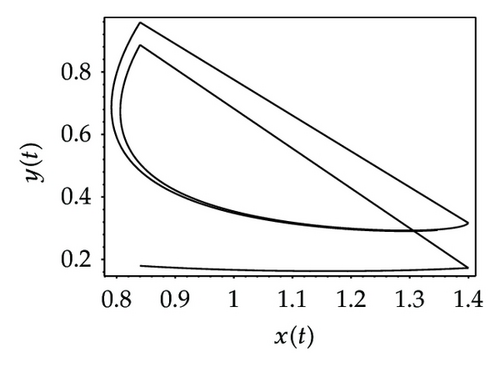
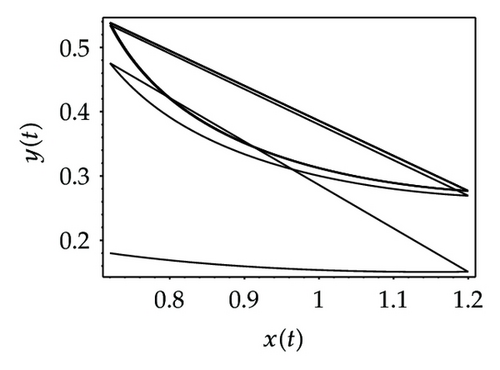
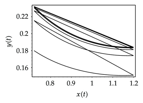
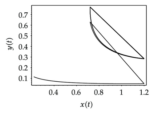
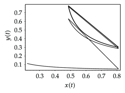
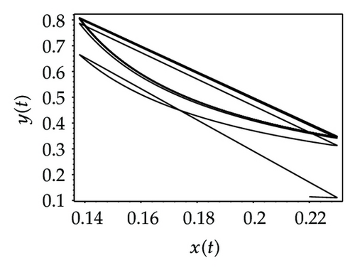
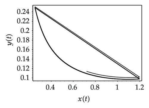
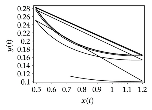
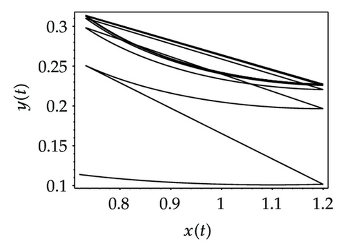
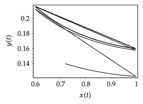
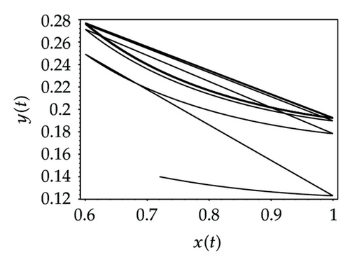
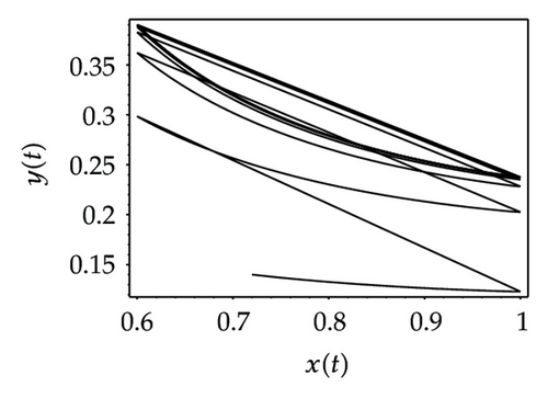
Choosing ι as a control parameter, the phase portraits of system (1.3) are shown in Figure 10 with different values ι, which not only indicate that the prey can be suppressed below certain level by using the impulsive state feedback strategy when the amount of the prey reaches the economic threshold h, but also indicate that it is more easy to control the amount of the prey below certain economic threshold h as ι increasing. On the other hand, if choosing h as a control parameter, we can see that more numbers of impulses are needed to make the system tend to a stable periodic solution, that is, it is more difficult to control the amount of the prey below economic threshold h as h is decreasing (see Figure 11). Figure 12 shows that it is more easy to control the amount of the prey under certain economic threshold h as q is increasing or p is increasing (see Figure 13).

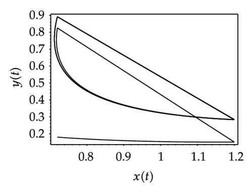
According to the above analysis, it is obvious that the prey can be well suppressed below certain level by using impulsive state feedback strategy for the fact that the system has stable periodic solution under some conditions. The key to the system with impulsive state feedback control is to give the suitable feedback state (the value of h) and the control parameters (p, q and ι) according to practice.

Acknowledgments

This work is supported by the National Natural Science Foundation of China (11171284), the Fujian Provincial Natural Science Foundation of China (2012J01012), the Fujian Provincial Education Fundation (JA12198), and the Scientific Research Foundation of Jimei University of China (ZC2011003).

References

1 Beddington J. R., Mutual interference between parasites or predators and its effect on searching efficency, Journal of Animal Ecology. (1975) 44, 331–340.
10.2307/3866
Web of Science® Google Scholar
2 DeAngelis D. L., Goldstein R. A., and O’Neill R. V., A model for trophic interaction, Ecology. (1975) 56, 881–892.
10.2307/1936298
Web of Science® Google Scholar
3 Xiang Z., Li Y., and Song X., Dynamic analysis of a pest management SEI model with saturation incidence concerning impulsive control strategy, Nonlinear Analysis. (2009) 10, no. 4, 2335–2345, https://doi.org/10.1016/j.nonrwa.2008.04.017, 2508441, ZBL1163.92332.
10.1016/j.nonrwa.2008.04.017
Google Scholar
4 Wei C. and Chen L., Eco-epidemiology model with age structure and prey-dependent consumption for pest management, Applied Mathematical Modelling. (2009) 33, no. 12, 4354–4363, https://doi.org/10.1016/j.apm.2009.03.015, 2567006, ZBL1179.34049.
10.1016/j.apm.2009.03.015
Web of Science® Google Scholar
5 Shi R., Jiang X., and Chen L., A predator-prey model with disease in the prey and two impulses for integrated pest management, Applied Mathematical Modelling. (2009) 33, no. 5, 2248–2256, https://doi.org/10.1016/j.apm.2008.06.001, 2494283, ZBL1185.34015.
10.1016/j.apm.2008.06.001
Web of Science® Google Scholar
6 Zhang H., Xu W., and Chen L., A impulsive infective transmission SI model for pest control, Mathematical Methods in the Applied Sciences. (2007) 30, no. 10, 1169–1184, https://doi.org/10.1002/mma.834, 2329638, ZBL1155.34328.
10.1002/mma.834
Web of Science® Google Scholar
7 Tang S., Xiao Y., Chen L., and Cheke R. A., Integrated pest management models and their dynamical behaviour, Bulletin of Mathematical Biology. (2005) 67, no. 1, 115–135, https://doi.org/10.1016/j.bulm.2004.06.005, 2204249.
10.1016/j.bulm.2004.06.005
PubMed Web of Science® Google Scholar
8 Zeng G., Chen L., and Sun L., Existence of periodic solution of order one of planar impulsive autonomous system, Journal of Computational and Applied Mathematics. (2006) 186, no. 2, 466–481, https://doi.org/10.1016/j.cam.2005.03.003, 2176360, ZBL1088.34040.
10.1016/j.cam.2005.03.003
Web of Science® Google Scholar
9 Jiang G. and Lu Q., Impulsive state feedback control of a predator-prey model, Journal of Computational and Applied Mathematics. (2007) 200, no. 1, 193–207, https://doi.org/10.1016/j.cam.2005.12.013, 2276825, ZBL1134.49024.
10.1016/j.cam.2005.12.013
Web of Science® Google Scholar
10 Jiang G., Lu Q., and Qian L., Complex dynamics of a Holling type II prey-predator system with state feedback control, Chaos, Solitons and Fractals. (2007) 31, no. 2, 448–461, https://doi.org/10.1016/j.chaos.2005.09.077, 2259769, ZBL1203.34071.
10.1016/j.chaos.2005.09.077
Web of Science® Google Scholar
11 Nie L., Peng J., Teng Z., and Hu L., Existence and stability of periodic solution of a Lotka-Volterra predator-prey model with state dependent impulsive effects, Journal of Computational and Applied Mathematics. (2009) 224, no. 2, 544–555, https://doi.org/10.1016/j.cam.2008.05.041, 2492887, ZBL1162.34007.
10.1016/j.cam.2008.05.041
Web of Science® Google Scholar
12 Abrams P. A., The fallacies of ratio-dependent predation, Ecology. (1994) 75, 1842–1850.
10.2307/1939644
Web of Science® Google Scholar
13 Haque M., A detailed study of the Beddington-DeAngelis predator-prey model, Mathematical Biosciences. (2011) 234, no. 1, 1–16, https://doi.org/10.1016/j.mbs.2011.07.003, 2894850.
10.1016/j.mbs.2011.07.003
PubMed Web of Science® Google Scholar
14 Baek H. K., Qualitative analysis of Beddington-DeAngelis type impulsive predator-prey models, Nonlinear Analysis. (2010) 11, no. 3, 1312–1322, https://doi.org/10.1016/j.nonrwa.2009.02.021, 2646548, ZBL1204.34062.
10.1016/j.nonrwa.2009.02.021
Google Scholar
15 Liu B., Tian Y., and Kang B., Dynamics on a Holling II predator-prey model with state-dependent impulsive control, International Journal of Biomathematics. (2012) 5, article 1260006.
Web of Science® Google Scholar
16 Zhao L., Chen L., and Zhang Q., The geometrical analysis of a predator-prey model with two state impulses, Mathematical Biosciences. (2012) 238, no. 2, 55–64, https://doi.org/10.1016/j.mbs.2012.03.011.
10.1016/j.mbs.2012.03.011
PubMed Web of Science® Google Scholar
17 Simeonov P. S. and Baĭnov D. D., Orbital stability of periodic solutions of autonomous systems with impulse effect, International Journal of Systems Science. (1988) 19, no. 12, 2561–2585, https://doi.org/10.1080/00207728808559591, 975426, ZBL0669.34044.
10.1080/00207728808547133
Web of Science® Google Scholar

Citing Literature

All articles

Periodic Solution of Prey-Predator Model with Beddington-DeAngelis Functional Response and Impulsive State Feedback Control

Abstract

1. Introduction

2. Definitions and Lemmas

3. Qualitative Analysis of System (1.3) without Impulsive Effects

4. Existence and Stability of Periodic Solutions of System (1.3)

4.1. Existence of Order One Periodic Solution

5. Numerical Analysis and Discussion

Acknowledgments

References

Citing Literature

Figures

References

Information

About Wiley Online Library

Help & Support

Opportunities

Connect with Wiley

Periodic Solution of Prey-Predator Model with Beddington-DeAngelis Functional Response and Impulsive State Feedback Control

Abstract

1. Introduction

2. Definitions and Lemmas

3. Qualitative Analysis of System (1.3) without Impulsive Effects

4. Existence and Stability of Periodic Solutions of System (1.3)

4.1. Existence of Order One Periodic Solution

5. Numerical Analysis and Discussion

Acknowledgments

References

Citing Literature

Figures

References

Related

Information